Processing, Training, and Deployment
Data preparation involves transforming raw data into a format that is suitable for further processing and analysis. This process includes several key steps: collecting, cleaning, and labeling the raw data to ensure it is ready for machine learning (ML) algorithms. Additionally, exploring and visualizing the data is essential.
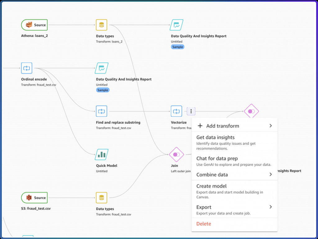
Data scientists and developers spend a significant amount of their time cleaning and preparing data before training machine learning (ML) models. This is necessary because real-world data cannot be used directly. It may contain missing values, duplicate entries, or various formats of the same information that need to be standardized. Furthermore, data often needs to be converted from one format to another to be compatible with machine learning algorithms. For instance, the XGBoost algorithm can only accept numerical data. Therefore, if the input data is in string or categorical format, it must be transformed into a numerical format before it can be utilized.
You can exclude a column from your model build by dropping it in the Build tab of the SageMaker Canvas application. Deselect the column you want to drop, and it isn’t included when building the model.
Encoding operation_status into numeric labels (e.g., 0 for legitimate, 1 for suspicious) is essential for compatibility with SageMaker’s built-in classification algorithms, which require numerical target variables.
SageMaker AI built-in algorithms typically expect numerical input features for training. Converting all fields to strings would degrade model performance and prevent proper feature engineering, especially for fields like payment_value and account_duration which are inherently numeric.
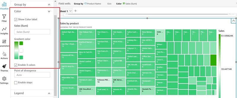
CountVectorizer
CountVectorizer from scikit-learn is a powerful tool for preprocessing text data in machine learning workflows. It transforms text data into a bag-of-words representation, which is crucial for feeding textual data into machine learning models. The key feature of CountVectorizer in this context is its ability to remove stopwords (commonly used, irrelevant words like “and,” “the,” and “in”) while still allowing rare words to be retained. This is important for tasks such as tag generation, where it is necessary to filter out common words that don’t provide meaningful information, while keeping infrequent but significant terms that can help improve the model’s accuracy.
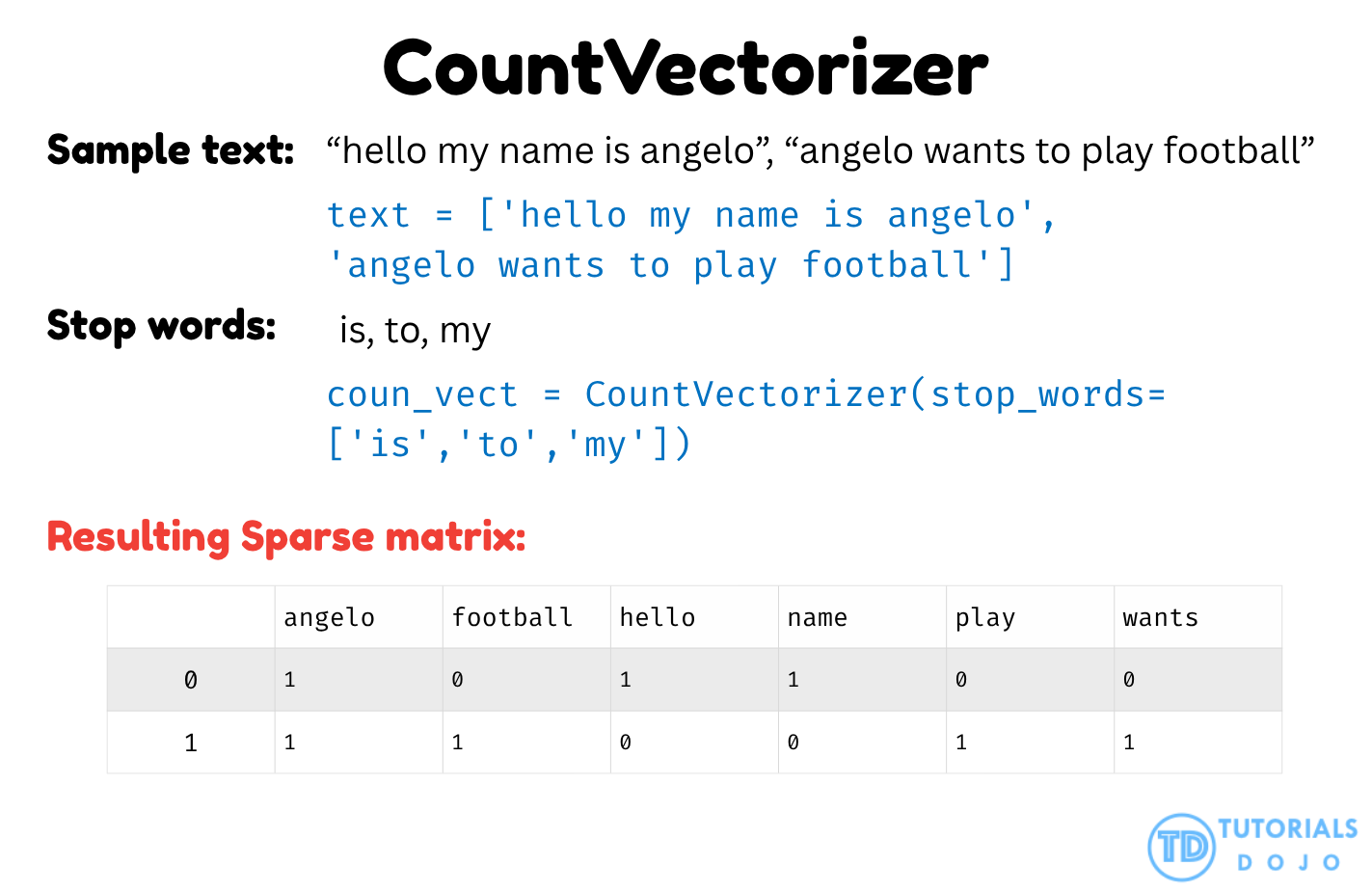
Integrating CountVectorizer, the process would follow these steps:
- Load the article data: The article data, stored in Amazon S3, is accessed for preprocessing.
- Preprocess the text:
CountVectorizeris applied to the article content, configured to remove stopwords while retaining rare words. - Cleaned data storage: The processed data, now free of stopwords and containing the important rare words, is stored back in S3 for use in Amazon SageMaker AI.
- Model training: Once the data is cleaned, it is fed into a machine learning model in SageMaker AI for training, which uses the refined text to generate more accurate tag predictions.
This process ensures that the article data is properly prepared for training a machine learning model, leveraging AWS services like SageMaker AI for model building and deployment.
CountVectorizer effectively removes stopwords while retaining rare, meaningful terms, ensuring that only relevant words are passed into the model. This makes it an ideal tool for text preprocessing, particularly for tasks like tag generation in machine learning models, where both the removal of common words and preservation of infrequent, valuable terms are critical. It can be applied to any textual data—such as articles, reviews, or product descriptions—within AWS services like SageMaker, helping improve model accuracy and relevance.
Amazon QuickSight
- Business analytics and visualizations in the cloud
- Serverless
- data source
- Redshift
- Aurora / RDS
- Athena
- EC2-hosted databases
- Files (S3 or on-premises)
- Excel
- CSV, TSV
- Common or extended log format
- AWS IoT Analytics
- Data preparation allows limited ETL
- SPICE
- Data sets are imported into SPICE
- Each user gets 10GB of SPICE
- Scales to hundreds of thousands of users
- Use cases
- Interactive ad-hoc exploration / visualization of data
- Dashboards and KPI’s
- Analyze / visualize data from:
- Logs in S3
- On-premise databases
- AWS (RDS, Redshift, Athena, S3)
- SaaS applications, such as Salesforce
- Any JDBC/ODBC data source
- Quicksight Q
- Machine learning-powered
- Answers business questions with Natural Language Processing
- Must set up topics associated with datasets
- Quicksight ML sights
- help uncover hidden insights and trends in your data. It does that by using an ML model that over time and with an increasing volume of data being fed into QuickSight, continually learns and improves its abilities to provide three key features (as of this writing):
- ML-powered anomaly detection – Detect outliers that show significant variance from the dataset. This can help identify significant changes in your business metrics such has low-performing stores or products, or top selling items.
- ML-powered forecasting – Detect trends and seasonality to forecast based on historical data. This can help project sales, orders, website traffic, and more.
- Autonarratives – Embed narratives in your dashboard to tell the story of your data in plain language. This can help convey a shared understanding of the data within your organization. You can use either the suggested autonarrative or you can customize the computations and language to meet your organization’s unique requirements.
- help uncover hidden insights and trends in your data. It does that by using an ML model that over time and with an increasing volume of data being fed into QuickSight, continually learns and improves its abilities to provide three key features (as of this writing):
- Quicksight Security
- Multi-factor authentication on your account
- VPC connectivity
- Row-level security
- Column-level security too (CLS) –Enterprise edition only
- Private VPC access
- Elastic Network Interface, AWS Direct Connect
- QuickSight Visual Types
- AutoGraph
- Bar Charts: comparison and distribution (histograms)
- A histogram is a type of chart that displays the distribution of numerical data by dividing it into intervals or bins. Each bar represents the frequency or count of data points falling within each interval, providing insights into the data’s distribution and density.
- Line graphs: changes over time
- Scatter plot, heat maps: correlation
- A heatmap is a visualization method that uses color gradients to represent values within a matrix. It displays data in a two-dimensional format where color intensity indicates the magnitude of values
- Pie graphs: aggregation
- Tree maps: Heirarchical Aggregation
- Pivot tables: tabular data
- KPIs: compare key value to its target value
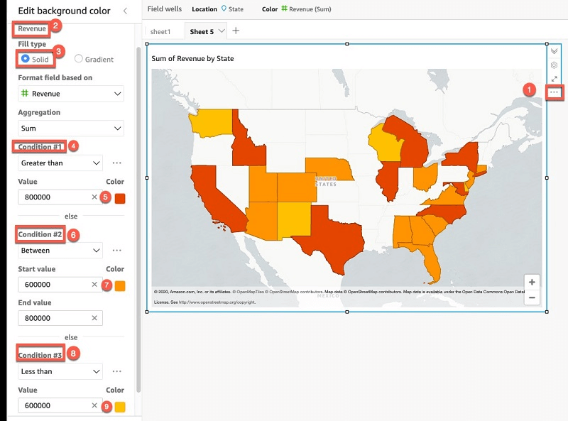
- Geospatial Charts (maps)
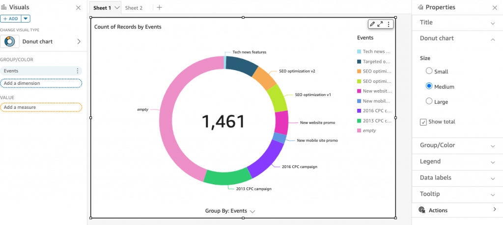
- Donut Charts: Percentage of Total Amount
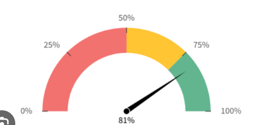
- Gauge Charts: Compare values in a measure
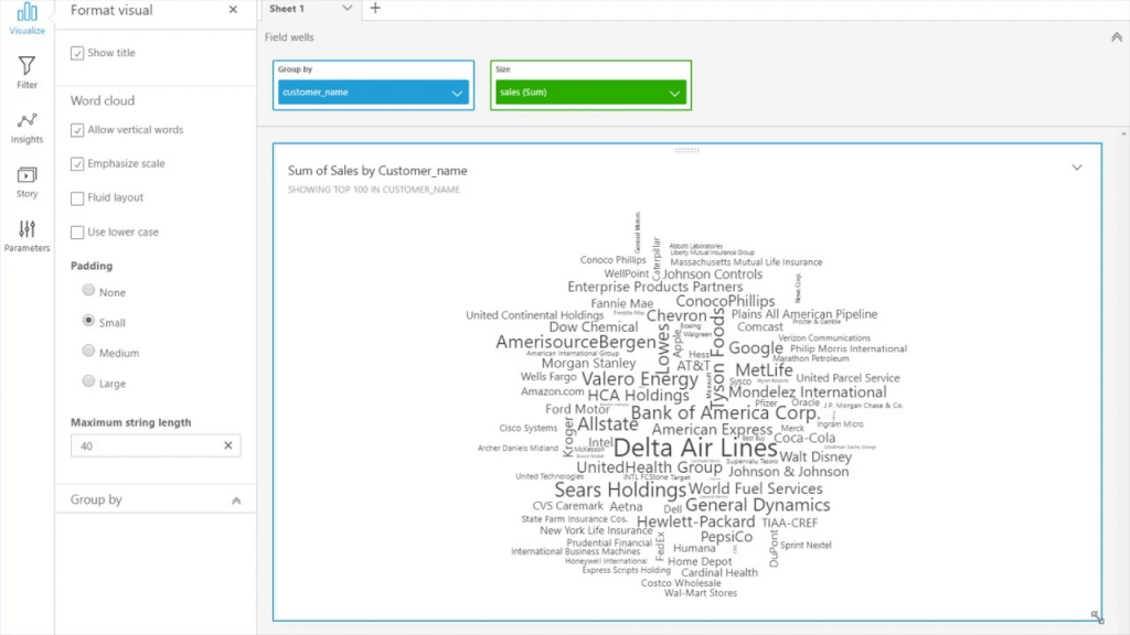
- Word Clouds: word or phrase frequency
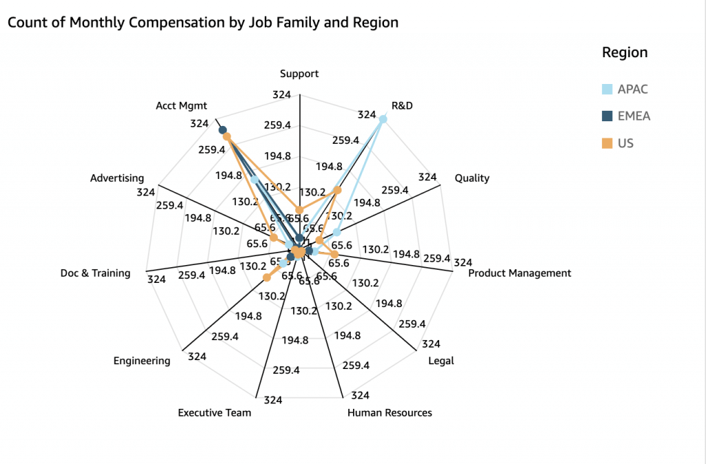
- Radar Chart
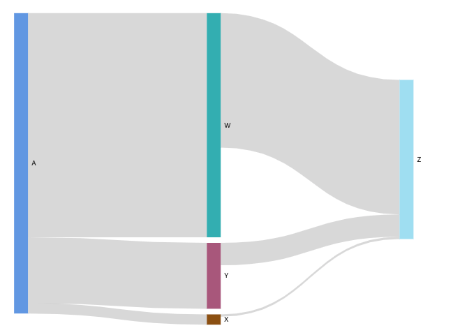
- Sankey diagrams: show flows from one category to another, or paths from one stage to the next
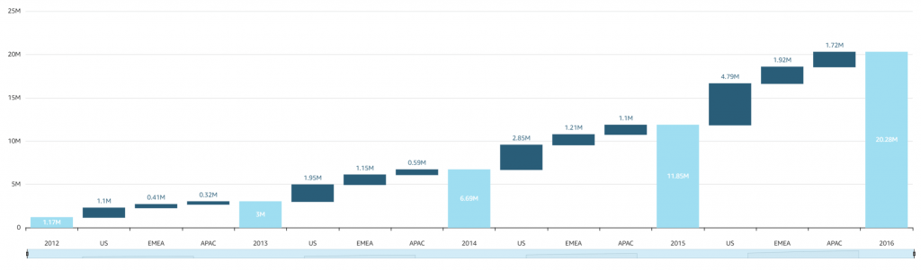
- Waterfall chart: visualize a sequential summation as values are added or subtracted
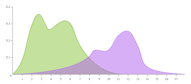
- (not provided) Density Plot
- aka Kernel Density Plot or Density Trace Graph
- visualises the distribution of data over a continuous interval or time period. This chart is a variation of a Histogram that uses kernel smoothing to plot values, allowing for smoother distributions by smoothing out the noise. The peaks of a Density Plot help display where values are concentrated over the interval.

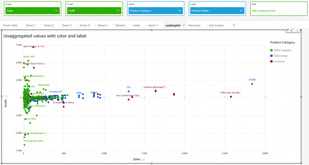

- [ 🧐QUESTION🧐 ] visualize recommendation results across four distinct dimensions
- visualize all four dimensions effectively:
- – X-axis: user’s interest score
- – Y-axis: product’s prior conversion rate
- – Color: product category
- – Size: number of impressions
- Scatter plots are ideal for this kind of multi-dimensional analysis, and SageMaker Canvas supports mapping both color and size attributes to data points.
- visualize all four dimensions effectively:
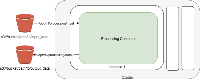
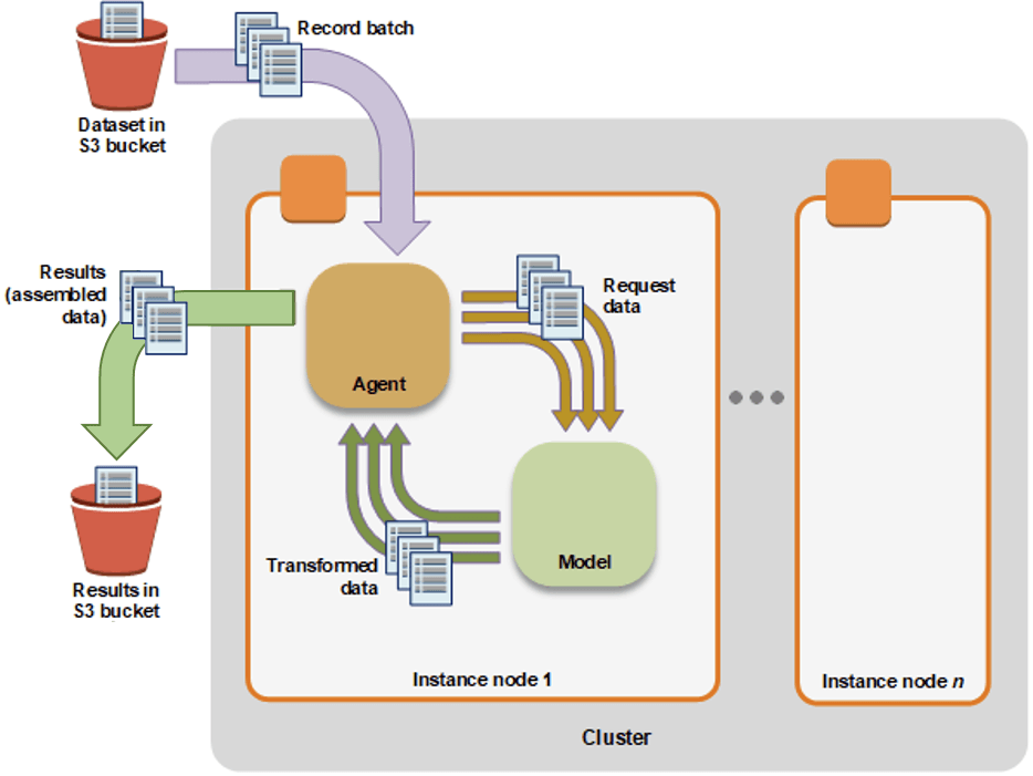
Amazon SageMaker Processing
- a fully managed service that simplifies the process of running data processing and model evaluation jobs
- run data pre and post processing, feature engineering, and model evaluation tasks on SageMaker
- ideal for more complex workflows such as feature engineering, model evaluation, and large-scale data transformation.
- built-in support for TensorFlow and Hugging Face’s Transformers and can directly interact with data stored in Amazon S3
- Input modes
- File mode
- source: S3 Bucket
- File mode downloads training data to a local directory in a Docker container.
- Fast file mode
- source: S3 Bucket
- At the start of training, fast file mode identifies the data files but does not download them. Training can start without waiting for the entire dataset to download.
- Fast file mode doesn’t support augmented manifest files.
- This means that your dataset no longer needs to fit into the training instance storage space as a whole, and you don’t need to wait for the dataset to be downloaded to the training instance before training starts.
- Pipe mode
- source: S3 Bucket
- Streaming can provide faster start times and better throughput than file mode.
- When you stream the data directly, you can reduce the size of the Amazon EBS volumes used by the training instance. Pipe mode needs only enough disk space to store the final model artifacts.
- data is pre-fetched from Amazon S3 at high concurrency and throughput, and streamed into a named pipe, which also known as a First-In-First-Out (FIFO) pipe for its behavior.
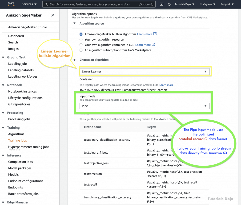
- can use the optimized protobuf recordIO data format for faster.
- Amazon S3 Express One Zone
- source: S3 Bucket
- high-performance, single Availability Zone storage class that can deliver consistent, single-digit millisecond data access for the most latency-sensitive applications
- Amazon FSx for Lustre
- source: FSx for Lustre
- scale to hundreds of gigabytes of throughput and millions of IOPS with low-latency file retrieval.
- Amazon EFS
- source: EFS
- File mode
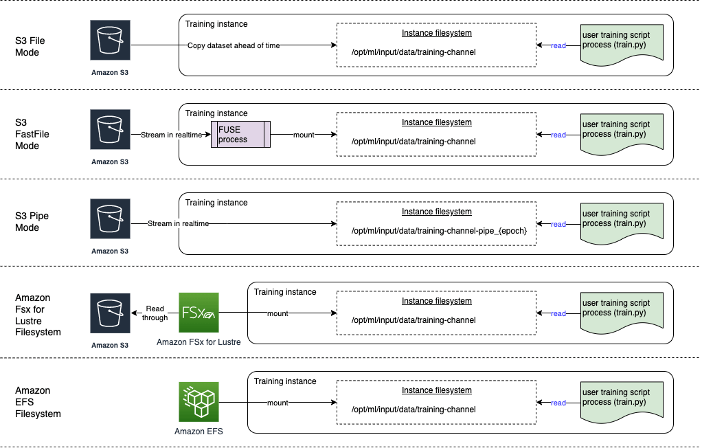
- for computer vision workloads using many small image files benefit more from FastFile mode, which allows random access to image data while streaming directly from Amazon S3. Using Pipe mode could complicate file handling within the training script without providing the same efficiency gains as FastFile mode for image-heavy tasks.
- Pipe mode is primarily optimized for sequential data reads, such as in natural language processing or large structured datasets.
Inference Model Deployment
- getting predictions, or inferences, from your trained machine learning models
- approaches
- Deploy a machine learning model in a low-code or no-code environment
- deploy pre-trained models using Amazon SageMaker JumpStart through the Amazon SageMaker Studio interface
- Use code to deploy machine learning models with more flexibility and control
- deploy their own models with customized settings for their application needs using the ModelBuilder class in the SageMaker AI Python SDK, which provides fine-grained control over various settings, such as instance types, network isolation, and resource allocation.
- Deploy machine learning models at scale
- use the AWS SDK for Python (Boto3) and AWS CloudFormation along with your desired Infrastructure as Code (IaC) and CI/CD tools
- Deploying a model to an endpoint
- ProductVariant for each model that you want to deploy
- VariantWeight to specify how much traffic you want to allocate to each model
- Cost optimization
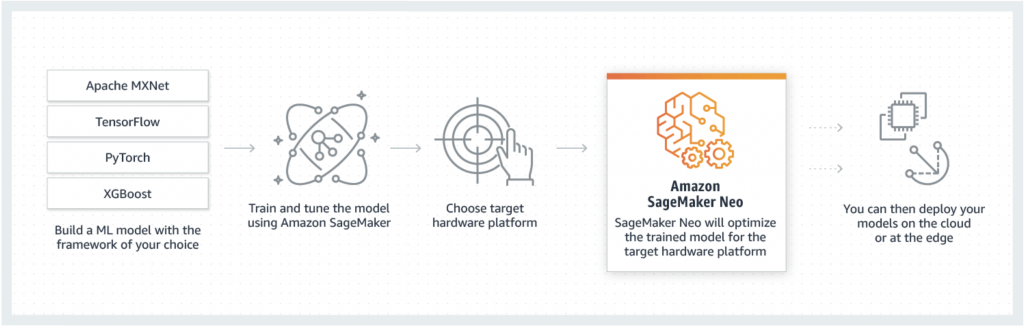
- Model performance optimization with SageMaker Neo.
- automatically optimizing models to run in environments like AWS Inferentia chips.
- Automatic scaling of Amazon SageMaker AI models.
- Use autoscaling to dynamically adjust the compute resources for your endpoints based on incoming traffic patterns, which helps you optimize costs by only paying for the resources you’re using at a given time.
- Model performance optimization with SageMaker Neo.
- Deploy a machine learning model in a low-code or no-code environment
- Inference Modes/Endpoint Type (deploying the model to an endpoint)
- Real-time inference
- inference workloads where you have real-time, interactive, low latency requirements
- short processing time (up to 60 seconds)
- multi-model endpoints are typically built on real-time inference architecture, which imposes a hard timeout limit (typically 60 seconds)
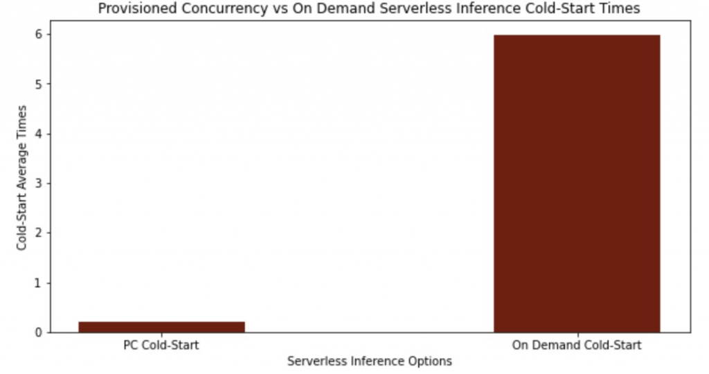
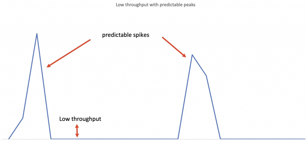
- (On-demand) Serverless inference
- workloads which have idle periods between traffic spurts and can tolerate cold starts
- without configuring or managing any of the underlying infrastructure
- compute resources are automatically launched and scaled based on traffic
- but, cannot configure a VPC for the endpoint
- also only support short processing time (up to 60 seconds)
- the memory requirements fit within the 6 GB memory and 200 maximum concurrency limits of serverless endpoints
- With “provisioned concurrency”, you can mitigate cold starts and get predictable
- keep the endpoints warm and ready to respond to requests instantaneously
- but it would cost
- performance characteristics for their workloads
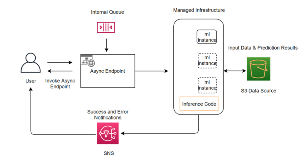
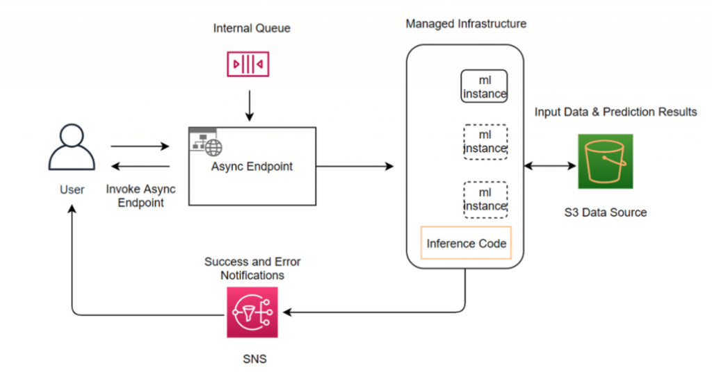
- Asynchronous inference
- queues incoming requests and processes them asynchronously
- requests with large payload sizes (up to 1GB), long processing times (up to 60 minutes), and near real-time latency requirements
- Creating an asynchronous inference endpoint is similar to creating real-time inference endpoints. You can use your existing SageMaker AI models and only need to specify the
AsyncInferenceConfigobject while creating your endpoint configuration with theEndpointConfigfield in theCreateEndpointConfigAPI. - Asynchronous Inference can be configured with an automatic scaling policy, enabling Amazon SageMaker to dynamically adjust the number of instances based on the volume of inference requests. The scaling policy uses predefined metrics to determine when to add or remove compute resources, maintaining performance during high demand while minimizing cost during idle periods. This elasticity ensures the infrastructure scales seamlessly to meet unpredictable workloads, providing high availability and consistent throughput for applications that process large data payloads or experience traffic surges.
- Real-time inference
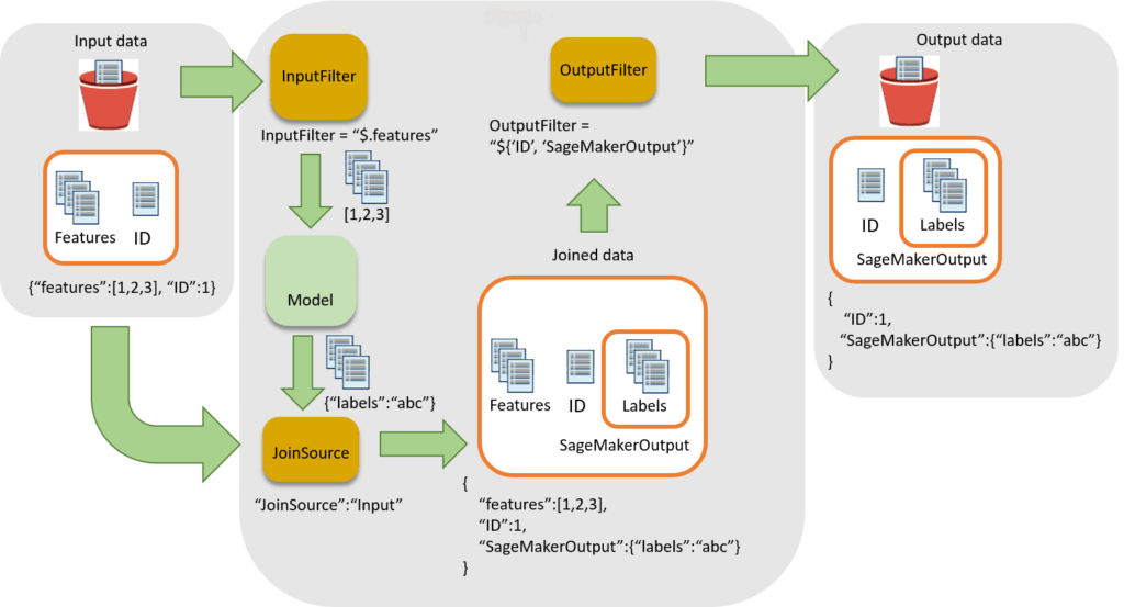
- Batch transform
- Preprocess datasets to remove noise or bias that interferes with training or inference from your dataset.
Get inferences from large datasets (minimum 100MB per dataset).- Run inference when you don’t need a persistent endpoint.
- appropriate for workloads that do not need to return an inference for each request to the model
- Associate input records with inferences to help with the interpretation of results.
- suitable for long-term monitoring and trend analysis
- especially when the task can be scheduled and does not require immediate real-time responses
- can handle processing jobs that take anywhere from a few minutes to several hours or even days, making it suitable for long-running jobs like daily sales predictions.
- primarily designed for offline, batch-style inference, not for interactive request/response workflows. Also, the payload size must not be greater than 100 MB.
- Deployment Safeguards
- Deployment Guardrails
- For asynchronous or real-time inference endpoints
- Controls shifting traffic to new models
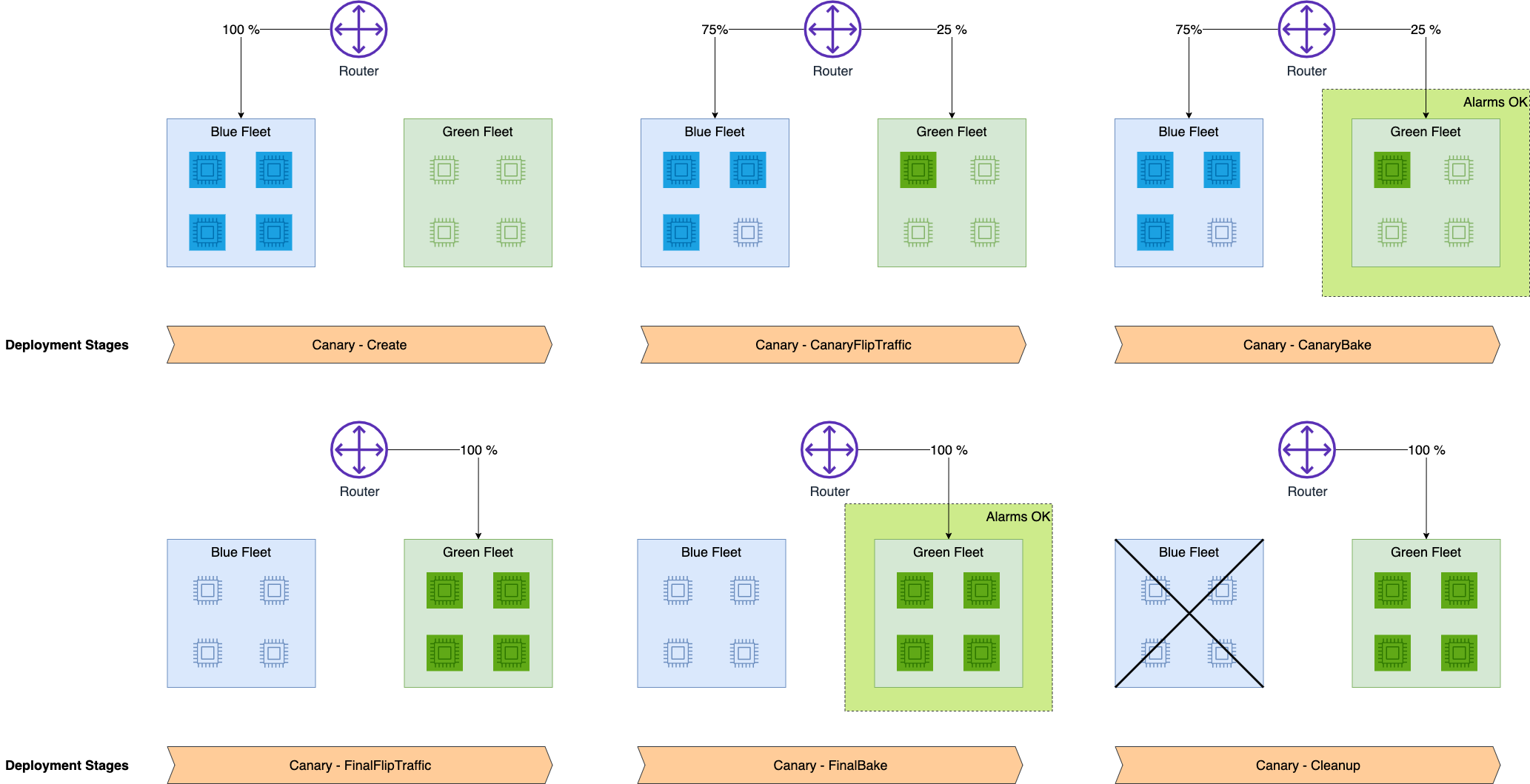
- Blue/Green Deployments
- ie “All at once”: shift everything, monitor, terminate blue fleet
- Canary
- allows you to deploy new versions of machine learning models or applications to a small subset of users or traffic
- Linear
- Shift traffic in linearly spaced steps
- does not provide the initial small-scale rollout and evaluation phase that Canary deployment offers
- (no good!) In-place
- update the application by using existing compute resources
- You stop the current version of the application. Then, you install and start the new version of the application
- Auto-rollbacks
- Shadow
- runs the new version alongside/parallelly the old version for testing without affecting live traffic
- Compare performance of shadow variant to production
- particularly valuable when user inference feedback isn’t necessary
- You monitor in SageMaker console and decide when to promote it
- Deployment Guardrails
| Use case 1 | Use case 2 | Use case 3 | |
|---|---|---|---|
| SageMaker AI feature | Use JumpStart in Studio to accelerate your foundational model deployment. | Deploy models using ModelBuilder from the SageMaker Python SDK. | Deploy and manage models at scale with AWS CloudFormation. |
| Description | Use the Studio UI to deploy pre-trained models from a catalog to pre-configured inference endpoints. This option is ideal for citizen data scientists, or for anyone who wants to deploy a model without configuring complex settings. | Use the ModelBuilder class from the Amazon SageMaker AI Python SDK to deploy your own model and configure deployment settings. This option is ideal for experienced data scientists, or for anyone who has their own model to deploy and requires fine-grained control. | Use AWS CloudFormation and Infrastructure as Code (IaC) for programmatic control and automation for deploying and managing SageMaker AI models. This option is ideal for advanced users who require consistent and repeatable deployments. |
| Optimized for | Fast and streamlined deployments of popular open source models | Deploying your own models | Ongoing management of models in production |
| Considerations | Lack of customization for container settings and specific application needs | No UI, requires that you’re comfortable developing and maintaining Python code | Requires infrastructure management and organizational resources, and also requires familiarity with the AWS SDK for Python (Boto3) or with AWS CloudFormation templates. |
| Recommended environment | A SageMaker AI domain | A Python development environment configured with your AWS credentials and the SageMaker Python SDK installed, or a SageMaker AI IDE such as SageMaker JupyterLab | The AWS CLI, a local development environment, and Infrastructure as Code (IaC) and CI/CD tools |
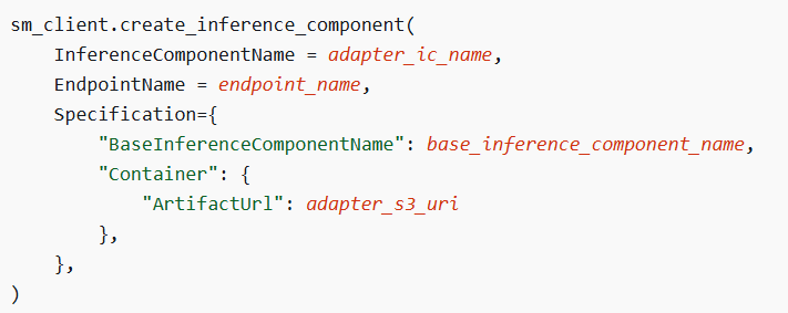
- [🧐QUESTION🧐 ] Fine-tune models with adapter inference components
- host your base foundation model by using a SageMaker AI inference component, you can fine-tune that base model with LoRA adapters by creating adapter inference components. When you create an adapter inference component, you specify the following:
- The base inference component that is to contain the adapter inference component. The base inference component contains the foundation model that you want to adapt. The adapter inference component uses the compute resources that you assigned to the base inference component.
- The location where you’ve stored the LoRA adapter in Amazon S3.
- After you create the adapter inference component, you can invoke it directly. When you do, SageMaker AI combines the adapter with the base model to augment the generated response.
- One cost-effective method for fine-tuning is Low-Rank Adaptation (LoRA). The key concept behind LoRA is that only a small portion of a large foundation model needs to be updated to adapt it for new tasks or domains. A LoRA adapter enhances the inference from a base foundation model by adding just a few additional adapter layers.
- Before you can create an adapter inference component, you must meet the following requirements:
– You must have a base inference component that includes the foundation model you wish to adapt. This component should be deployed to a SageMaker AI endpoint.
– You need to have a LoRA adapter model, with the model artifacts stored astar.gzfile in Amazon S3. When creating the adapter inference component, you will specify the S3 URI of these artifacts.
The example below demonstrates how to create an adapter inference component and link it to a base inference component. - Deploy the base model once to a SageMaker AI real-time endpoint, then for each region, use a separate adapter inference component containing the region’s Low-Rank Adaptation (LoRA) adapter artifacts and invoke the same endpoint by specifying the region’s adapter
- host your base foundation model by using a SageMaker AI inference component, you can fine-tune that base model with LoRA adapters by creating adapter inference components. When you create an adapter inference component, you specify the following:
- [🧐QUESTION🧐 ] introduce new model into production without inference endpoint change
-
CreateEndpointConfigcreates an endpoint configuration that SageMaker hosting services uses to deploy models. In the configuration, you identify one or more models, created using theCreateModelAPI, to deploy and the resources that you want SageMaker to provision. Then you call theCreateEndpointAPI. - In the request, you define a
ProductionVariant, for each model that you want to deploy. EachProductionVariantparameter also describes the resources that you want SageMaker to provision. This includes the number and type of ML compute instances to deploy. - If you are hosting multiple models, you also assign a
VariantWeightto specify how much traffic you want to allocate to each model. For example, suppose that you want to host two models, A and B, and you assign traffic weight 2 for model A and 1 for model B. SageMaker distributes two-thirds of the traffic to Model A, and one-third to model B. ProductionVariantidentifies a model that you want to host and the resources chosen to deploy for hosting it. If you are deploying multiple models, tell SageMaker how to distribute traffic among the models by specifying variant weights.InitialVariantWeightdetermines initial traffic distribution among all of the models that you specify in the endpoint configuration. The traffic to a production variant is determined by the ratio of theVariantWeightto the sum of allVariantWeightvalues across all ProductionVariants.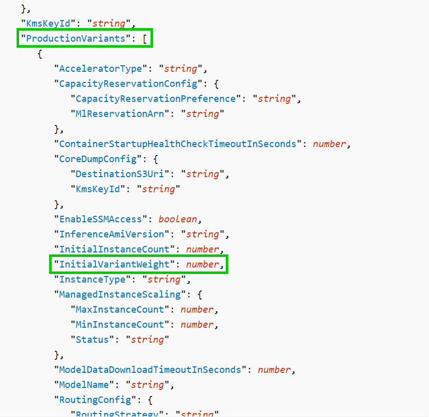
-
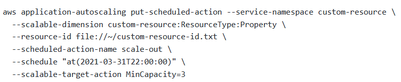
Scheduled scaling
allows you to automatically adjust your application’s capacity based on predictable load changes by creating scheduled actions that increase or decrease capacity at specific times. This helps you proactively scale your application to match anticipated load changes.
For instance, if you notice a regular weekly traffic pattern where load increases in the middle of the week and declines toward the weekend, you can configure a scaling schedule in Application Auto Scaling that aligns with this pattern:
- On Wednesday morning, one scheduled action can increase capacity by raising the previously set minimum capacity of the scalable target.
- On Friday evening, another scheduled action can decrease capacity by lowering the previously set maximum capacity of the scalable target.
These scheduled scaling actions help you optimize both costs and performance. This way, your application will have sufficient capacity to handle peak traffic on Wednesdays but will avoid unnecessary over-provisioning at other times.
You can also combine scheduled scaling with scaling policies to benefit from both proactive and reactive scaling approaches. After a scheduled scaling action is executed, the scaling policy can still determine if further capacity adjustments are needed. This ensures that you have enough capacity to manage your application’s load, while also ensuring that the current capacity remains within the minimum and maximum limits set by your scheduled action.
You can set up scheduled actions to scale resources either one time or on a recurring schedule. Once a scheduled action is executed, your scaling policy can still dynamically adjust scaling based on changes in workload. Please note that scheduled scaling can only be managed through the AWS CLI or the Application Auto Scaling API.
using variants behind the same endpoint. A variant consists of a machine learning (ML) instance along with the serving components specified in a SageMaker AI model. You can have multiple variants associated with a single endpoint, and each variant can utilize a different instance type or a different SageMaker AI model. This allows them to autoscale independently of one another.
The models within these variants can be trained using different datasets, algorithms, ML frameworks, or any combination of these factors. All the variants share the same inference code. SageMaker AI supports two types of variants: production variants and shadow variants.
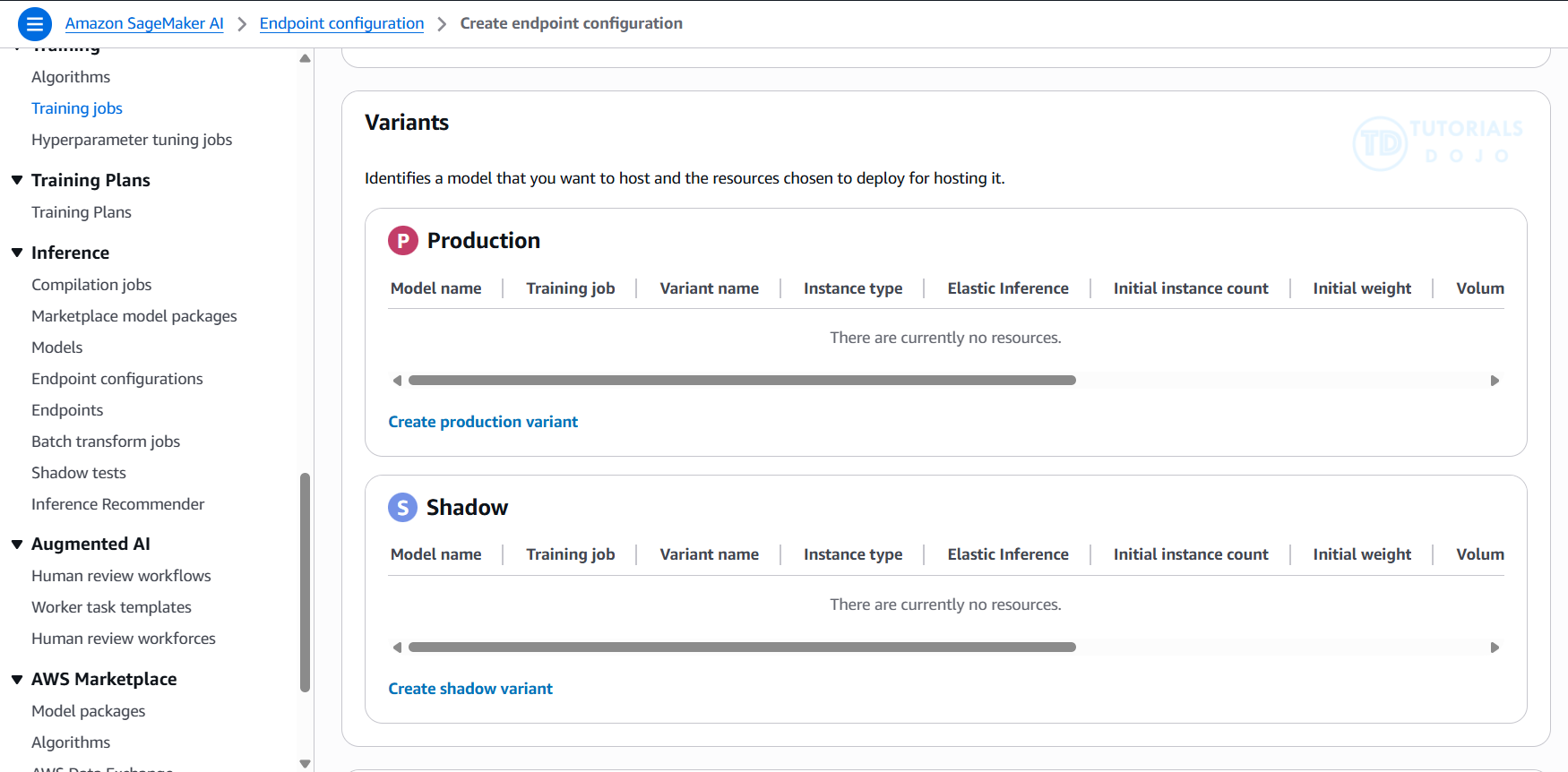
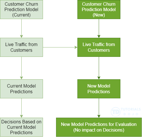
If you have several production variants behind an endpoint, you can allocate a portion of your inference requests to each variant. Each request will be directed to only one of the production variants, and that variant will provide the response to the caller. This setup allows you to compare the performance of the production variants relative to one another. You can also create a shadow variant that corresponds to a production variant behind an endpoint. A portion of the inference requests directed to the production variant is also sent to the shadow variant. The responses generated by the shadow variant are logged for comparison, but they are not returned to the caller. This setup allows you to test the performance of the shadow variant without exposing the caller to its responses..
In production ML workflows, data scientists and engineers often seek to enhance model performance through various methods. These methods include automatic model tuning with SageMaker AI, training on additional or more recent data, improving feature selection, and using updated instances and serving containers. To find the best performing model for inference requests, you can utilize production variants to compare different models, instances, and containers.
With SageMaker AI multi-variant endpoints, you can distribute endpoint invocation requests across multiple production variants by specifying the traffic distribution for each variant. Alternatively, you can directly invoke a specific variant for each request. This topic explores both approaches for testing ML models.
Amazon SageMaker Multi-Model Endpoints
- deploy multiple models behind a single endpoint.
- multiple models that need to be served simultaneously
- Utilize the same set of resources and a shared serving container, which helps reduce hosting costs and deployment overhead. Amazon SageMaker manages the loading of models in memory and scales them based on the traffic patterns to your endpoint.
- or perform A/B testing between different models.
- It is typically used for use cases where many smaller models need to be loaded dynamically from Amazon S3 at inference time, not for production-grade version transitions.
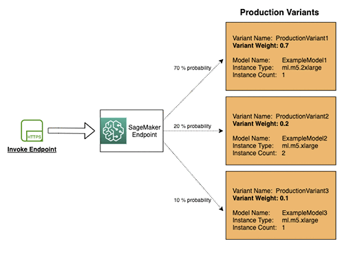
Multi-model endpoints provide a scalable and cost-effective solution to deploying large numbers of models. They use a shared serving container that is enabled to host multiple models. This reduces hosting costs by improving endpoint utilization compared with using single-model endpoints. It also reduces deployment overhead because Amazon SageMaker manages loading models in memory and scaling them based on the traffic patterns to them.
Multi-model endpoints are fully managed and highly available to serve traffic in real-time. You can easily invoke a specific model by specifying the target model name as a parameter in your prediction request.
Deployment Safeguards and Optimization
Deployment Guardrails
- For asynchronous or real-time inference endpoints
- Controls shifting traffic to new models
- “Blue/Green Deployments”
- All at once: shift everything, monitor, terminate blue fleet
- Canary: shift a small portion of traffic and monitor
- Linear: Shift traffic in linearly spaced steps
- “Blue/Green Deployments”
- Auto-rollbacks
Shadow Tests
- Compare performance of shadow variant to production
- You monitor in SageMaker console and decide when to promote it
- Shadow testing is a valuable technique for validating model performance under real traffic conditions, but it simply mirrors requests to the new model without influencing live predictions
Optimizing FM Deployments
- SageMaker AI offers single and multi-model endpoints
- More generally, multi-container endpoints
- Each endpoint supports deployment guardrails, VPC, network isolation
- You can train/tune a model in SageMaker AI, and deploy through Bedrock
- You use Bedrock Custom Model Import for this
- Now your inference is serverless ☺
- SageMaker AI Inference Components
- Each model gets its own scaling policy
- Cross-region inference profiles
- For endpoints on Bedrock
- EC2 Auto Scaling Groups
- Load balancing in front of SageMaker AI endpoints
- Available model servers with SageMaker AI
- TorchServe
- DJL Serving (Deep Java Library)
- Deep Learning Containers
- DJL was created by Amazon, so more likely to show up on exam
- Triton Inference Server
- Use asynchronous inference if latency isn’t important
- SageMaker AI async endpoints
- Your own queue with SNS / SQS
- Model compression
- Quantization (of model weights)
- Quantization is the process of converting continuous or highly precise values into a smaller, finite set of discrete values, essentially “rounding” data to fit into predefined buckets, reducing file size and computational load while sacrificing some accuracy. It’s crucial in signal processing (turning analog waves into digital numbers), quantum physics (energy existing in fixed levels), and AI/Machine Learning (making large models run faster on smaller devices) by using lower-precision numbers (like int8 instead of float32).
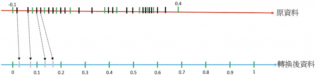
- Quantile Binning Transformation is a process used to discover non-linearity in the variable’s distribution by grouping observed values together. It won’t help normalize features with wide-ranging differences.The quantile binning processor takes two inputs, a numerical variable and a parameter called bin number, and outputs a categorical variable. The purpose is to discover non-linearity in the variable’s distribution by grouping observed values together.
In many cases, the relationship between a numeric variable and the target is not linear (the numeric variable value does not increase or decrease monotonically with the target). In such cases, it might be useful to bin the numeric feature into a categorical feature representing different ranges of the numeric feature. Each categorical feature value (bin) can then be modeled as having its own linear relationship with the target. For example, let’s say you know that the continuous numeric feature account_age is not linearly correlated with likelihood to purchase a book. You can bin age into categorical features that might be able to capture the relationship with the target more accurately.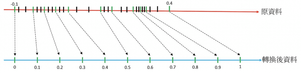
- Pruning
- Model pruning aims to remove weights that don’t contribute much to the training process. Weights are learnable parameters: they are randomly initialized and optimized during the training process. During the forward pass, data passes through the model. The loss function evaluates model output given the labels; during the backward pass, weights are updated to minimize the loss. To do so, the gradients of the loss with respect to the weights are computed, and each weight receives a different update.
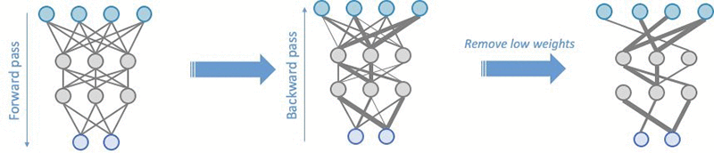
- Model pruning aims to remove weights that don’t contribute much to the training process. Weights are learnable parameters: they are randomly initialized and optimized during the training process. During the forward pass, data passes through the model. The loss function evaluates model output given the labels; during the backward pass, weights are updated to minimize the loss. To do so, the gradients of the loss with respect to the weights are computed, and each weight receives a different update.
- Knowledge distillation
- A smaller model is trained from a larger model
- Quantization (of model weights)
- Avoid premature optimization
- Measure your performance, costs, resource utilization
- Don’t solve problems that don’t exist!
SageMaker Experiments
- Organize, capture, compare, and search your ML jobs
- use to automatically create ML experiments by using different combinations of data, algorithms, and parameters
- allows the engineer to automatically track each model’s run, hyperparameters, and results, making it easier to evaluate multiple algorithms and choose the best-performing model
- The purpose of SageMaker Experiments is to simplify the creation of experiments, populate them with trials, add tracking and lineage information, and conduct analytics across trials and experiments.
- A SageMaker AI experiment consists of runs, and each run consists of all the inputs, parameters, configurations, and results for a single model training interaction.
- You can log parameters and metrics from a remote function using either the @remote decorator or the
RemoteExecutorAPI. - It allows the team to systematically track and compare preprocessing parameters, sample sizes, and resulting model metrics across multiple runs. SageMaker Experiments is purpose-built for organizing ML workflows and analyzing how input variations affect model performance.
- [ NOT ] SageMaker Debugger is primarily designed to monitor and profile training jobs, not preprocessing scripts. It captures internal model states like tensors and gradients, but it doesn’t support logging PySpark parameters or tracking preprocessing variations in a structured way.
- [ NOT ] Model Monitor is typically used for post-deployment monitoring of data drift and model quality in production endpoints. It does not track preprocessing parameters or support experimentation during training or processing jobs.
- [ NOT ] Autopilot automates preprocessing and model selection using its own internal logic. It does not support custom PySpark scripts or manual control over feature engineering parameters, which are essential for the team’s experimentation goals.
| Purpose | Service | Note |
|---|---|---|
| Finetune – Preprocessing parameters | Experiments | PySpark |
| Finetune – Sample size | Experiments | |
| Training jobs | Debugger | |
| Productions (Data drift, model quality) | Model Monitor | |
| Automations | Autopilot | |
Amazon SageMaker Automatic Model Tuning (AMT)
- hyperparameter optimization of the model
- “HyperParameter Tuning Job” that trains as many combinations as you’ll allow
- It learns as it goes
- Best Practices
- Don’t optimize too many hyperparameters at once
- Limit your ranges to as small a range as possible
- Use logarithmic scales when appropriate
- Don’t run too many training jobs concurrently
- This limits how well the process can learn as it goes
- Make sure training jobs running on multiple instances report the correct objective metric in the end
- Strategies
- Grid Search: chooses combinations of values from the range of categorical values that you specify. Only categorical parameters are supported when using the grid search strategy
- Grid search simply tests every combination of hyperparameters in a predefined range, which makes it highly inefficient for large search spaces. It typically consumes excessive computational resources and time because every job runs to completion regardless of performance. This brute-force method is useful for small experiments but does not support early stopping or adaptive resource allocation, making it unsuitable for efficiently optimizing complex models.
- Random Search
- While it can sometimes find good configurations faster than grid search, it still lacks any built-in mechanism to stop poorly performing jobs early. It simply runs each trial to completion, which typically wastes resources on weak configurations. Random search does not provide the intelligent resource management and adaptive early stopping offered by Hyperband, making it less cost-effective for large-scale tuning tasks.
- Bayesian optimization: treats as regression problem
- efficiently explores the hyperparameter space by building a probabilistic model of performance
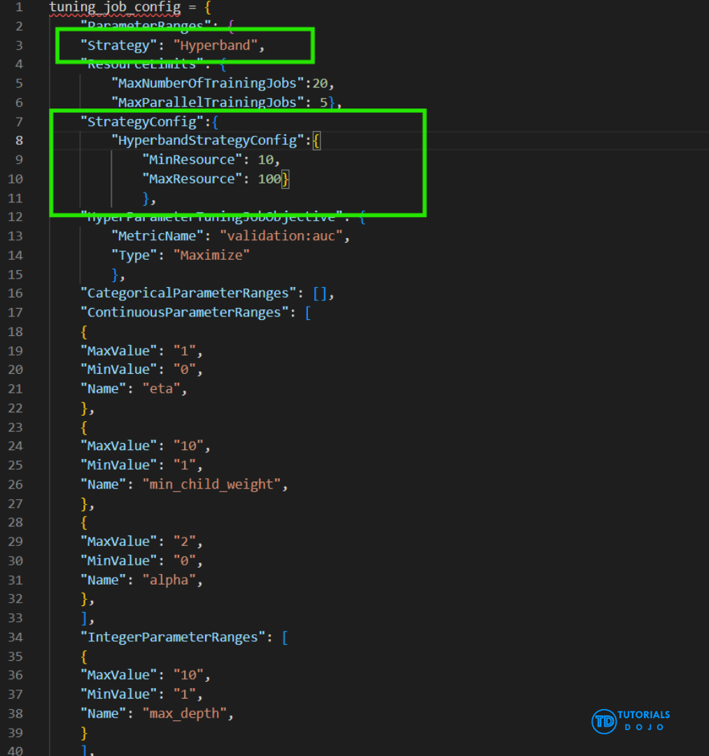
- Hyperband
- Grid Search: chooses combinations of values from the range of categorical values that you specify. Only categorical parameters are supported when using the grid search strategy
- Stop the training jobs that a hyperparameter tuning job launches early when they are not improving significantly as measured by the objective metric. Stopping training jobs early can help reduce compute time and helps you avoid overfitting your model.
- use early stopping to compare the current objective metric (accuracy) against the median of the running average of the objective metric
- Use warm start to start a hyperparameter tuning job using one or more previous tuning jobs as a starting point. The results of previous tuning jobs are used to inform which combinations of hyperparameters to search over in the new tuning job.
- Reasons
- To gradually increase the number of training jobs over several tuning jobs based on results after each iteration.
- To tune a model using new data that you received.
- To change hyperparameter ranges that you used in a previous tuning job, change static hyperparameters to tunable, or change tunable hyperparameters to static values.
- Types
- IDENTICAL_DATA_AND_ALGORITHM
- uses the same input data and training image as the parent tuning jobs
- use the same training data as you used in a previous hyperparameter tuning job, but you want to increase the total number of training jobs or change ranges or values of hyperparameters
- TRANSFER_LEARNING
- use different input data, hyperparameter ranges, and other hyperparameter tuning job parameters than the parent tuning jobs
- IDENTICAL_DATA_AND_ALGORITHM
- Reasons
- The Hyperband strategy in SageMaker AI is designed to make hyperparameter tuning more efficient by intelligently allocating computational resources. Hyperband automatically stops poorly performing training jobs early while continuing to allocate more resources to promising configurations. This approach reduces training time and GPU costs without compromising model quality. Hyperband is particularly useful when working with large datasets or complex models, as it dynamically balances the exploration of the hyperparameter space with the exploitation of the best-performing trials.
Automate key machine learning tasks and use no-code or low-code solutions
- SageMaker Canvas
- No-code machine learning for business analysts
- Capabilities for tasks
- such as data preparation, feature engineering, algorithm selection, training and tuning, inference, and more.
- Upload csv data (csv only for now), select a column to predict, build it, and make predictions
- Can also join datasets
- Classification or regression
- Automatic data cleaning
- Missing values
- Outliers
- Duplicates
- Share models & datasets with SageMaker Studio
- Custom models: for numeric prediction, categories prediction, and time series forecasting
- Ready-to-use models
- Sentiment analysis
- Entities extraction
- Language detection
- Personal information detection
- Document analysis
- Document queries
- Object detection in images
- Text detection in images
- Expense analysis
- Identity document analysis
- The Finer Points
- Local file uploading must be configured “by your IT administrator.”
- Set up an S3 bucket with appropriate CORS permissions
- Can integrate with Okta SSO
- Canvas lives within a SageMaker Domain that must be manually updated
- Import from Redshift can be set up
- Time series forecasting must be enabled via IAM
- Can run within a VPC
- Local file uploading must be configured “by your IT administrator.”
- SageMaker Autopilot (has been integrated into Canvas)
- Automates:
- Algorithm selection
- Data preprocessing
- Model tuning
- All infrastructure
- It does all the trial & error for you
- More broadly this is called AutoML
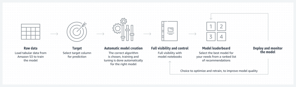
- Wokflow
- Load data from S3 for training
- Select your target column for prediction
- Automatic model creation
- Model notebook is available for visibility & control
- Model leaderboard
- Ranked list of recommended models
- You can pick one
- Deploy & monitor the model, refine via notebook if needed
- Can add in human guidance
- With or without code in SageMaker Studio or AWS SDK’s
- Problem types:
- Binary classification
- Multiclass classification
- Regression
- Algorithm Types:
- Linear Learner
- XGBoost
- Deep Learning (MLP’s)
- Ensemble mode
- Data must be tabular CSV or Parquet
- Training Modes ???
- HPO (Hyperparameter optimization)
- Ensembling
- Auto
- Explainability ???
- Integrates with SageMaker Clarify
- Transparency on how models arrive at predictions
- Feature attribution
- Uses SHAP Baselines / Shapley Values
- Research from cooperative game theory
- Assigns each feature an importance value for a given prediction
- Automates:
- SageMaker JumpStart
- One-click models and algorithms from model zoos
- provides pre-built models and end-to-end solutions for common machine learning use cases
- Over 150 open source models in NLP, object detections, image classification, etc.
- also provides solution templates that set up infrastructure for common use cases, and executable example notebooks for machine learning with SageMaker AI
- NOT allow testing different algorithms and custom training
- [ 🧐QUESTION🧐 ] Combine Model Registry with Canvas
- To enable access to the fine-tuned model created outside of Amazon SageMaker, the AI developer must first register the model in the SageMaker Model Registry. This action ensures that the model is properly versioned and cataloged, making it available for use in SageMaker Canvas. Once the model is registered, the data specialist can access it through the no-code interface of Canvas, experiment with its text-generation capabilities, and perform editorial tasks. However, it is also important that the data specialist has the necessary permissions to access the S3 bucket where the model artifacts are stored. These permissions ensure that the model artifacts are available for use in Canvas.
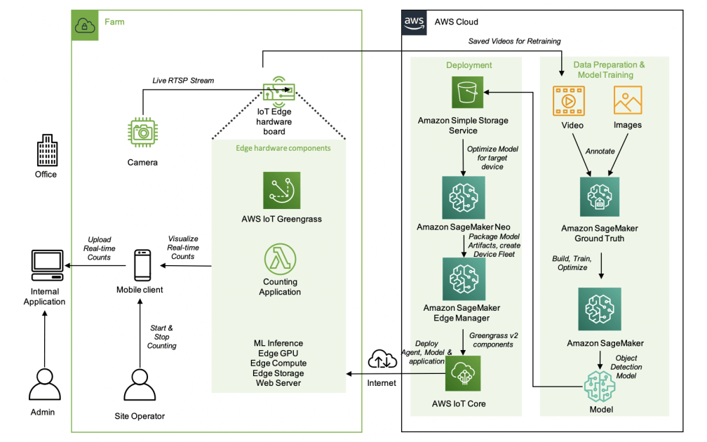
- [ 🧐QUESTION🧐 ] Object Dectection in IoT
- The object detection algorithm identifies and locates all instances of objects within an image from a predefined set of object categories. It takes an image as input and outputs both the category to which the object belongs and a confidence score reflecting the likelihood of the object’s classification. Additionally, the algorithm predicts the object’s location and size using a rectangular bounding box.
- Amazon SageMaker AI Object Detection utilizes the Single Shot Multibox Detector (SSD) algorithm. This algorithm is based on a convolutional neural network (CNN) that is pretrained for classification tasks. SSD leverages the outputs from intermediate layers of the network as features for detection.
- Various CNNs, such as VGG and ResNet, have achieved great performance on the image classification task. Object detection in Amazon SageMaker AI supports both VGG-16 and ResNet-50 as a base network for SSD. The algorithm can be trained in full training mode or in transfer learning mode. In full training mode, the base network is initialized with random weights and then trained on user data. In transfer learning mode, the base network weights are loaded from pretrained models.
- The object detection algorithm uses standard data augmentation operations, such as flip, rescale, and jitter, on the fly internally to help avoid overfitting.
- The AWS IoT Greengrass client software, also called AWS IoT Greengrass Core software, runs on Windows and Linux-based distributions, such as Ubuntu or Raspberry Pi OS, for devices with ARM or x86 architectures. With AWS IoT Greengrass, you can program devices to act locally on the data they generate, run predictions based on machine learning models, and filter and aggregate device data. AWS IoT Greengrass enables local execution of AWS Lambda functions, Docker containers, native OS processes, or custom runtimes of your choice.
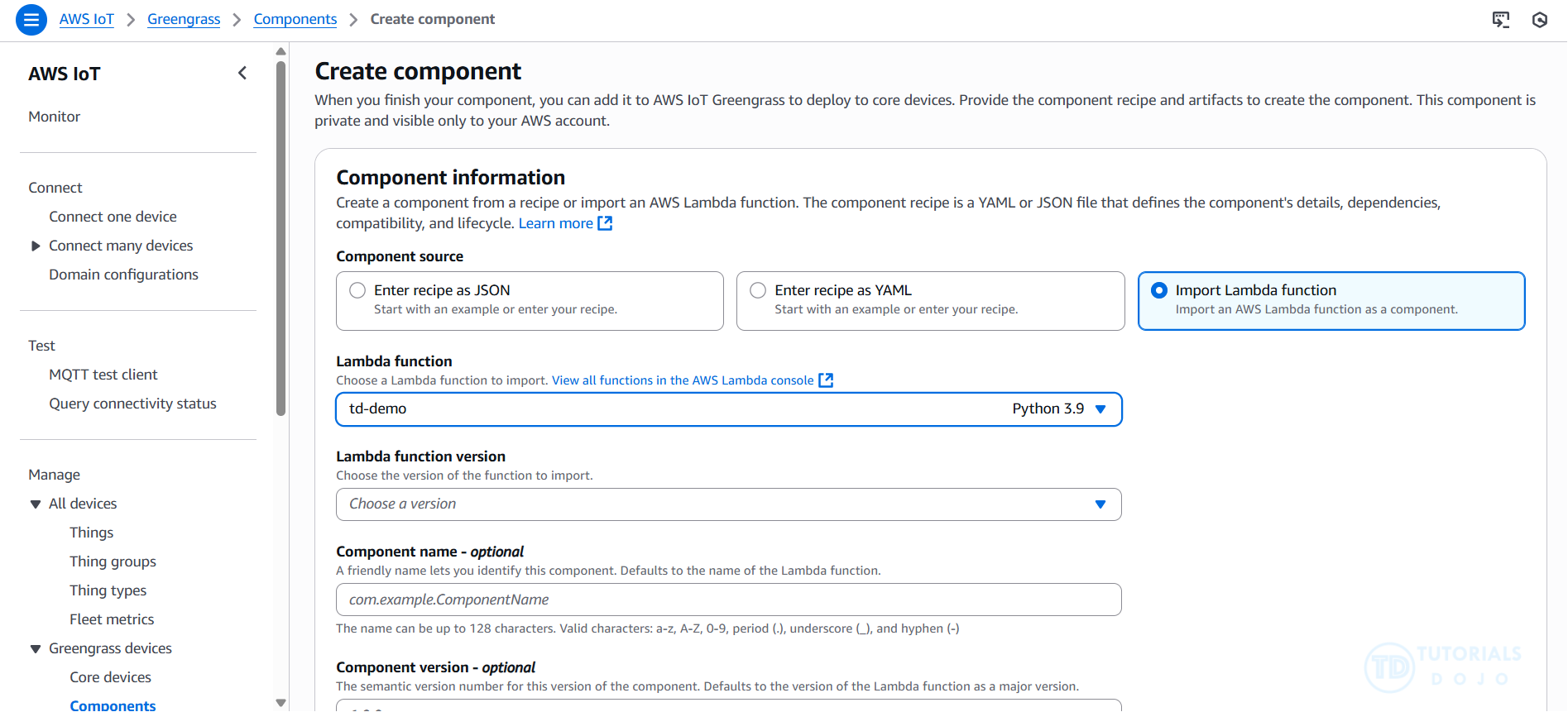
AWS IoT Greengrass provides pre-built software modules called components that let you easily extend edge device functionality. AWS IoT Greengrass components enable you to connect to AWS services and third-party applications at the edge. After you develop your IoT applications, AWS IoT Greengrass enables you to remotely deploy, configure, and manage those applications on your fleet of devices in the field.
AWS IoT Greengrass provides the following machine learning components that you can deploy to supported devices to perform machine learning inference using models trained in Amazon SageMaker AI or with your own pre-trained models that are stored in Amazon S3.
AWS provides the following categories of machine learning components:
– Model component – Contains machine learning models as Greengrass artifacts.
– Runtime component – Contains the script that installs the machine learning framework and its dependencies on the Greengrass core device.
– Inference component – Contains the inference code and includes component dependencies to install the machine learning framework and download pre-trained machine learning models.
| Forecast/Interferencing Tasks | ||
| Regression | Autopilot | |
| Classification | Autopilot, XGBoost | |
| Time series | DeepAR | RNN, suitable for large, multi-series datasets |
| Time series | Prophet | an additive regression model with a piecewise linear or logistic growth curve trend, more focus on seasonal, weekly, daily univariate time series. |
To enable access to the fine-tuned model created outside of Amazon SageMaker, the AI developer must first register the model in the SageMaker Model Registry. This action ensures that the model is properly versioned and cataloged, making it available for use in SageMaker Canvas. Once the model is registered, the data specialist can access it through the no-code interface of Canvas, experiment with its text-generation capabilities, and perform editorial tasks. However, it is also important that the data specialist has the necessary permissions to access the S3 bucket where the model artifacts are stored. These permissions ensure that the model artifacts are available for use in Canvas.
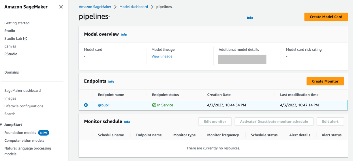
Amazon SageMaker AI is a fully managed machine learning service that simplifies the process of building, training, and deploying models at scale. One of its key components for production-grade MLOps is the SageMaker Model Registry, which provides a centralized repository for storing, tracking, and managing approved model versions. The registry helps ensure that only validated models are promoted to production environments, maintaining compliance, traceability, and governance across the machine learning lifecycle. By integrating with CI/CD pipelines, the Model Registry allows organizations to automate approval workflows and deployment steps seamlessly.
Amazon SageMaker real-time inference endpoints are designed for low-latency, high-throughput predictions from deployed models. These endpoints can automatically scale to handle variable traffic and support multiple deployment strategies such as blue/green, shadow, and rolling updates. They enable teams to test new model versions safely without impacting uptime or user experience. This makes them ideal for mission-critical workloads like fraud detection, financial scoring, and recommendation systems where every millisecond of latency matters.
For workloads requiring high computational performance, SageMaker supports accelerated instance types such as ml.g5 , ml.p4d , or ml.p5 . These GPU-powered instances are optimized for deep learning inference and training tasks that require parallel processing and high throughput. By selecting the right instance family, organizations can balance cost, speed, and resource efficiency based on their model’s complexity and real-time performance requirements.
Finally, Reserved Instances (RIs) in SageMaker allow companies to optimize cost efficiency by committing to a consistent amount of instance usage over a one- or three-year term. RIs provide significant discounts compared to on-demand pricing, making them ideal for long-running, stable production endpoints. For businesses deploying always-on inference services, such as financial models or healthcare analytics, RIs help maintain predictable costs while ensuring the performance needed for continuous real-time inference.
A multi-model endpoint enables multiple models to be hosted on a single SageMaker endpoint, optimizing infrastructure efficiency and cost. It is typically used for use cases where many smaller models need to be loaded dynamically from Amazon S3 at inference time, not for production-grade version transitions. This approach lacks built-in traffic control, health monitoring, and automatic rollback features, which are essential for safely deploying new versions in real-time applications.
Shadow testing is a valuable technique for validating model performance under real traffic conditions, but it simply mirrors requests to the new model without influencing live predictions. It is primarily used to gather metrics, compare model outputs, and detect potential regressions before a production rollout. However, this method does not perform any real traffic shifting or live user impact testing.
The batch transform feature is designed for offline inference on large static datasets, not for live, real-time traffic. It is typically used to preprocess data or generate predictions at scale, such as scoring historical records or evaluating model performance before deployment. While it can help validate the model’s accuracy, it only performs inference in batch mode and cannot dynamically shift traffic or monitor endpoint performance. Promoting the model directly after a batch test would bypass critical safety mechanisms, such as canary validation and rollback, which are vital for production stability.
Amazon FSx for Lustre is a high-performance file system designed for workloads that require fast, parallel access to large datasets, such as ML training, high-performance computing (HPC), and data analytics. When linked to an Amazon S3 bucket, FSx for Lustre automatically presents S3 objects as files in a file system, enabling SageMaker training jobs to read data at file system speeds while maintaining S3 as the source of truth. Any data written back to FSx can also be automatically exported to S3, ensuring seamless integration between object storage and high-performance file systems without data duplication or complex migration.
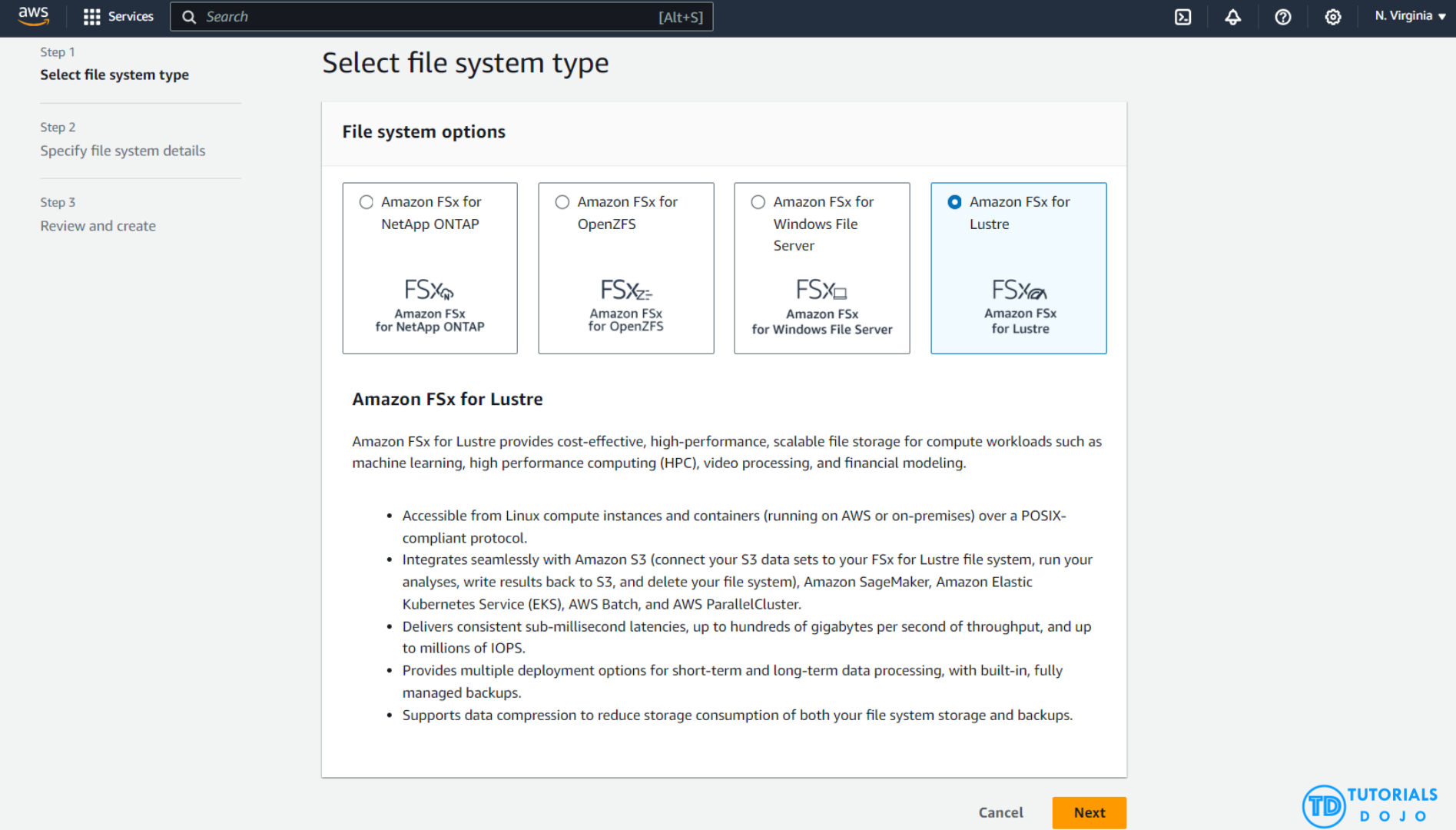
Amazon S3 serves as a durable, scalable, and cost-effective data lake for ML workloads. It is often used as the central repository for raw and processed data, model artifacts, and annotations. While S3 provides excellent durability and scalability, it is an object storage service, not a file system, meaning that sequential downloads of thousands of files can become a bottleneck during high-frequency read operations. By integrating S3 with FSx for Lustre, organizations can preserve the cost and durability benefits of S3 while gaining file system-level performance.
SageMaker Ground Truth
- Ground Truth
- Sometimes you don’t have training data at all, and it needs to be generated by humans first.
- Example: training an image classification model. Somebody needs to tag a bunch of images with what they are images of before training a neural network
- Ground Truth manages humans who will label your data for training purposes
- Ground Truth creates its own model as images are labeled by people
- As this model learns, only images the model isn’t sure about are sent to human labelers
- This can reduce the cost of labeling jobs by 70%
- Ground Truth Plus
- Turnkey solution
- “Our team of AWS Experts” manages the workflow and team of labelers
- You fill out an intake form
- They contact you and discuss pricing
- You track progress via the Ground Truth Plus Project Portal
- Get labeled data from S3 when done
- Other ways to generate training labels
- Rekognition
- AWS service for image recognition
- Automatically classify images
- Comprehend
- AWS service for text analysis and topic modeling
- Automatically classify text by topics, sentiment
- Any pre-trained model or unsupervised technique that may be helpful
- Rekognition
SageMaker Model Monitor
- Get alerts on quality deviations on your deployed models (via CloudWatch)
- Visualize data drift
- Example: loan model starts giving people more credit due to drifting or missing input features
- Detect anomalies & outliers
- Detect new features
- No code needed
- Data is stored in S3 and secured
- Monitoring jobs are scheduled via a Monitoring Schedule
- Metrics are emitted to CloudWatch
- CloudWatch notifications can be used to trigger alarms
- You’d then take corrective action (retrain the model, audit the data)
- Integrates with Tensorboard, QuickSight, Tableau
- Or just visualize within SageMaker Studio
- Monitoring Types:
- Drift in data quality
- Relative to a baseline you create
- “Quality” is just statistical properties of the features
- changes in the statistical properties of input data over time
- Drift in model quality (accuracy, etc)
- Works the same way with a model quality baseline
- Can integrate with Ground Truth labels
- impacts the model’s understanding of the relationship between inputs and outputs
- Bias drift
- Feature attribution drift
- Based on Normalized Discounted Cumulative Gain (NDCG) score
- This compares feature ranking of training vs. live data
- Drift in data quality
| Drift Types | Meaning | Activity | Class |
|---|---|---|---|
| Data quality drift | production data distribution differs from that used for training – the statistical properties of input data change | missing values or errors in the data | ModelDataQualityMonitor; DefaultModelMonitor |
| Model quality drift | predictions that a model makes differ from actual Ground Truth labels that the model attempts to predict | monitor the performance of a model by comparing the predictions that the model makes with the actual ground truth labels that the model attempts to predict | ModelPerformanceMonitor |
| Bias drift | introduction of bias due to change in production data distribution or application – starts to favor specific groups over others because of changes in data distribution or model parameters | statistical changes in the data distribution, even if the data has high quality | ModelBiasMonitor |
| Feature attribution drift | ranking of individual features changed from training data to live data – the significance of various features in a predictive model changes | detect feature attribution drift by comparing how the ranking of the individual features changed from training data to live data | ModelExplainabilityMonitor |
- [ 🧐QUESTION🧐 ] production-safe way to monitor the model’s performance over time and automatically re-train the model with the newly collected data
- With Model Monitor, you can set up the following monitoring options:
- Continuous monitoring with a real-time endpoint.
- Continuous monitoring with a batch transform job that runs regularly.
- On-schedule monitoring for asynchronous batch transform jobs.
- With Model Monitor, you can set up alerts to notify you of any deviations in model quality. Early and proactive detection of these deviations allows you to take corrective actions efficiently. You can take actions such as retraining models, auditing upstream systems, or addressing quality issues, all without the need for manual monitoring or additional tooling. Model Monitor offers prebuilt monitoring capabilities that require no coding, while also providing the flexibility to customize your analysis through coding if desired.
- Amazon SageMaker Model Monitor automatically oversees machine learning (ML) models in production and alerts you to any quality issues that arise. It employs rules to detect drift in your models and notifies you when this occurs.
- With Model Monitor, you can set up the following monitoring options:
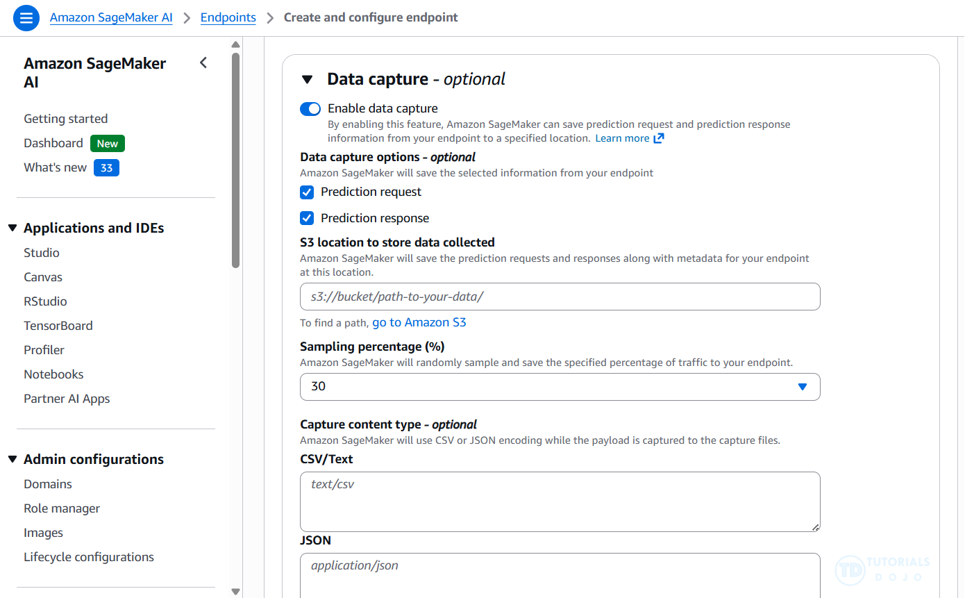
- To log the inputs to your endpoint and the inference outputs from your deployed model, you can enable a feature called Data Capture. This feature is commonly used to record information for training, debugging, and monitoring purposes. Amazon SageMaker Model Monitor automatically analyzes the captured data and compares the metrics from this data to a baseline that you establish for the model.
- [ NOT ] SageMaker Ground Truth + SageMaker Pipelines
- Ground Truth typically requires human or automated labeling, which adds latency and cost. While Pipelines help automate retraining, the need for labeled data increases overhead compared to using already captured inference data.
- [ NOT ] SageMaker Debugger
- Debugger is primarily designed for monitoring training jobs, not deployed endpoints. It doesn’t natively support inference-time monitoring or automatic retraining triggers based on production data, making it unsuitable for this use case.
- [ NOT ] SageMaker Experiments
- SageMaker Experiments is meant for tracking and comparing training runs, not for monitoring deployed models or collecting inference data. It lacks built-in mechanisms to detect drift or trigger retraining based on real-time production performance.
- [ NOT ] SageMaker Ground Truth + SageMaker Pipelines

The change from training data to live data appears significant. The feature ranking has completely reversed. Similar to the bias drift, the feature attribution drifts might be caused by a change in the live data distribution and warrant a closer look into the model behavior on the live data. Again, the first step in these scenarios is to raise an alarm that a drift has happened.
| Feature | Attribution in training data | Attribution in live data |
|---|---|---|
| SAT score | 0.70 | 0.10 |
| GPA | 0.50 | 0.20 |
| Class rank | 0.05 | 0.70 |
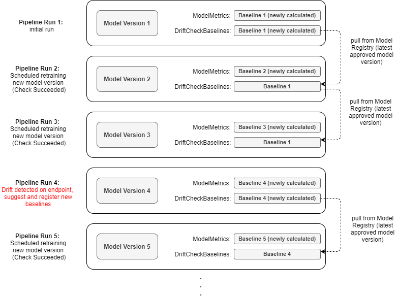
In production environments, Model Monitor compares incoming data to a baseline dataset to detect anomalies. If the baseline is outdated, even with a newly trained model, it will continue to flag violations, as the model’s output no longer aligns with the old reference data.

In this scenario, the engineer has deployed a new model and is still facing monitoring violations because Model Monitor is referencing an outdated baseline. To resolve this, the baseline dataset needs to be updated to reflect the new traffic. Performing a new baseline job with the latest training dataset will ensure that Model Monitor compares current data to a relevant baseline, eliminating false violations and allowing for accurate performance monitoring.
By regenerating the baseline with the updated data and configuring Model Monitor to use it, the engineer will resolve the violations and ensure that monitoring is aligned with the current data. This solution ensures that SageMaker Model Monitor can properly detect and flag real issues without being affected by mismatched or outdated baseline data.
SageMaker Clarify
- SageMaker Clarify detects potential bias
- i.e., imbalances across different groups / ages / income brackets
- With ModelMonitor, you can monitor for bias and be alerted to new potential bias via CloudWatch
- SageMaker Clarify also helps explain model behavior
- Understand which features contribute the most to your predictions
- Pre-training Bias Metrics
- Class Imbalance (CI)
- One facet (demographic group) has fewer training values than another
- Difference in Proportions of Labels (DPL)
- Imbalance of positive outcomes between facet values
- Kullback-Leibler Divergence (KL), Jensen-Shannon Divergence(JS)
- How much outcome distributions of facets diverge
- Lp-norm (LP)
- P-norm difference between distributions of outcomes from facets
- Total Variation Distance (TVD)
- L1-norm difference between distributions of outcomes from facets
- Kolmogorov-Smirnov (KS)
- Maximum divergence between outcomes in distributions from facets
- Conditional Demographic Disparity (CDD)
- Disparity of outcomes between facets as a whole, and by subgroups
- Class Imbalance (CI)

- [ 🧐QUESTION🧐 ] identify, measure, and explain potential bias across both the dataset and the model outputs
- SageMaker Clarify, a feature designed to help teams detect bias in data and models while improving interpretability.
- Clarify can analyze pre-training datasets to identify potential sources of bias, such as unequal representation of demographic or categorical attributes, and can also assess post-training model behavior to detect disparities in prediction outcomes.
- By quantifying fairness metrics and providing detailed statistical insights, Clarify helps teams build models that are more equitable and aligned with regulatory and ethical standards.
- In addition to bias detection, SageMaker Clarify provides explainability reports through SHAP (SHapley Additive exPlanations) values, which measure how much each feature contributes to an individual prediction. This capability enables organizations to understand why a model made a specific decision, which is crucial in regulated industries such as finance, healthcare, and e-commerce. The explainability reports can be used for compliance documentation, internal audits, or improving model design by highlighting overly influential or redundant features.
- [ NOT ] SageMaker Data Wrangler is primarily designed for data preparation, exploration, and transformation, not for bias detection or fairness evaluation. While it can help manually rebalance datasets, it does not provide automated bias metrics or explainability tools.
- [ NOT ] SageMaker Model Monitor is typically used to detect data drift, model quality degradation, and performance anomalies in deployed machine learning models. It simply observes operational metrics and changes in feature distribution over time. However, it does not evaluate fairness or explainability metrics. It complements Clarify for ongoing monitoring, but cannot identify or quantify bias within data or predictions on its own.
- [ NOT ] Amazon Personalize is a fully managed personalization service that optimizes recommendations based on user interactions and historical data. While it can indirectly influence recommendation fairness through retraining and user feedback loops, it primarily focuses on improving recommendation accuracy, rather than auditing or quantifying model bias.
- Amazon SageMaker Clarify helps identify and measure potential bias in datasets and models. It provides detailed insights into pretraining bias (bias present in the data before the model is trained) and posttraining bias (bias in the model’s predictions). In this scenario, Clarify was used to reveal that the training dataset was heavily skewed toward legitimate claims, indicating a class imbalance problem. Such an imbalance can cause a model to learn biased decision boundaries, where it favors the majority class and underrepresents the minority class during prediction.
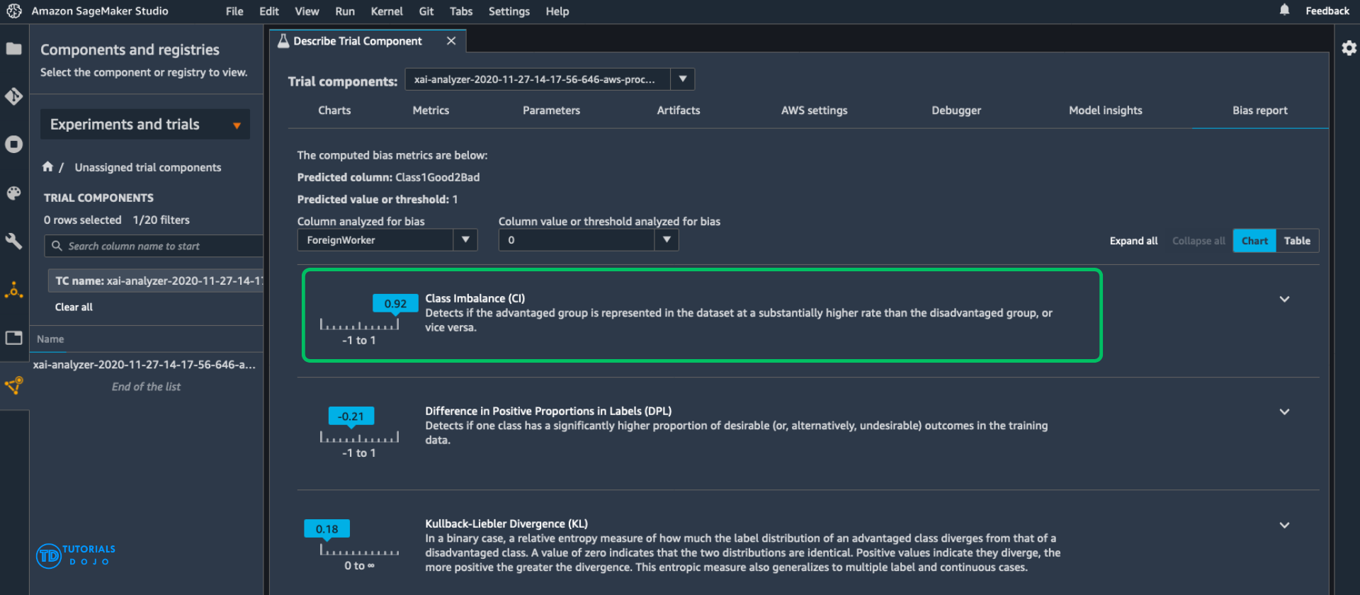
- Class Imbalance (CI) occurs when one or more classes in a dataset contain significantly fewer examples than others. This imbalance can lead to poor model generalization and biased outcomes, particularly when the model is trained using accuracy-based metrics that favor the majority class. To mitigate CI, practitioners can use techniques such as oversampling the minority class, undersampling the majority class, generating synthetic data (for example, using SMOTE), or applying class weights during training. Addressing class imbalance is critical in real-world applications, like fraud detection or medical diagnosis, where identifying rare events accurately is far more important than overall accuracy.
- [ 🧐QUESTION🧐 ] Overfitting with XGBoost
- Lower “
max_depth“ - [ NOT ] Reducing
min_child_weightlowers the minimum number of observations required to create a new leaf node, which typically increases the model’s complexity. Doing so encourages the model to just create more splits, even for insignificant variations in data, leading to deeper trees and more overfitting. - [ NOT ] Increasing
colsample_bytreeallows the model to use a larger fraction of available features for each tree, which primarily increases feature diversity rather than reducing overfitting. Although this can sometimes help stabilize training, it does not directly limit model complexity. In fact, allowing more features per tree can simply make the model more likely to overfit on correlated inputs if dominant features consistently drive splits.
- Lower “
Model Registry
Lineage Tracking
SageMaker on the Edge
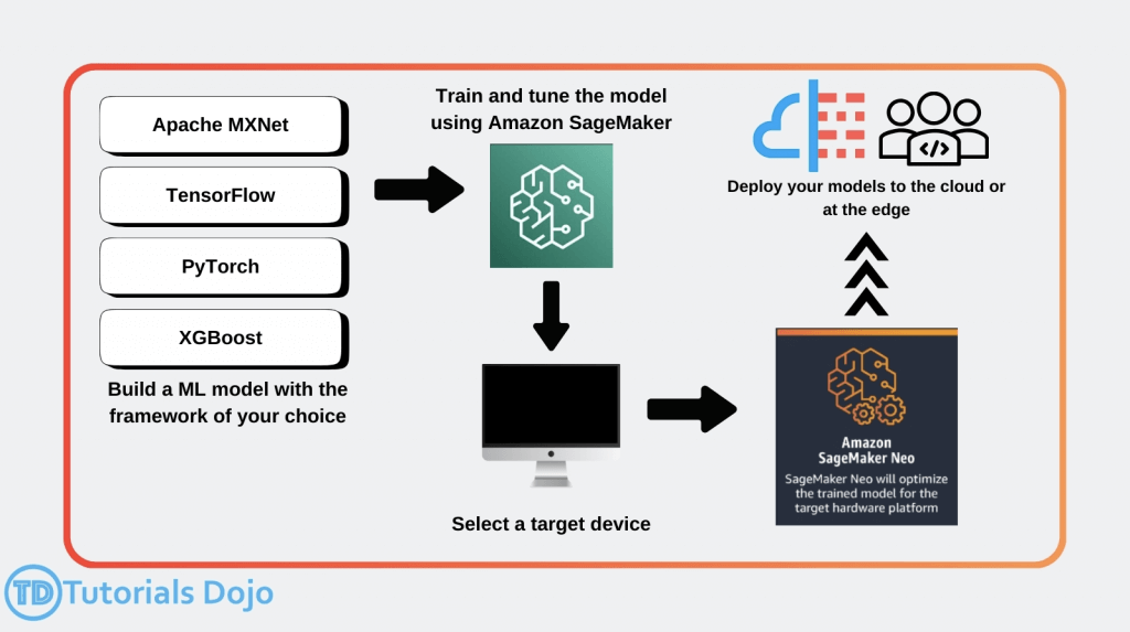
- SageMaker Neo
- Train once, run anywhere
- so it’s for “enhances models’ performance after training”
- used to optimize machine learning models for inference on different hardware platforms, including edge devices
- Edge devices
- ARM, Intel, Nvidia processors
- Optimizes code for specific devices
- Tensorflow, MXNet, PyTorch, ONNX, XGBoost, DarkNet, Keras
- Consists of a compiler and a runtime
- models are compiled into an optimized binary, allowing them to run with significantly lower latency and reduced compute resources, making it ideal for applications requiring fast decision-making, such as object detections.
- Train once, run anywhere
- Neo + AWS IoT Greengrass
- Neo-compiled models can be deployed to an HTTPS endpoint
- Hosted on C5, M5, M4, P3, or P2 instances
- Must be same instance type used for compilation
- OR! You can deploy to IoT Greengrass
- This is how you get the model to an actual edge device
- Inference at the edge with local data, using model trained in the cloud
- Uses Lambda inference applications
- Neo-compiled models can be deployed to an HTTPS endpoint
Pipelines
S3 Transfer Acceleration enhances upload and download speeds for long-distance transfers over the public internet, primarily benefiting cross-region or geographically distributed clients. Enabling Transfer Acceleration would not meaningfully reduce intra-region data access time or address the sequential download bottleneck.
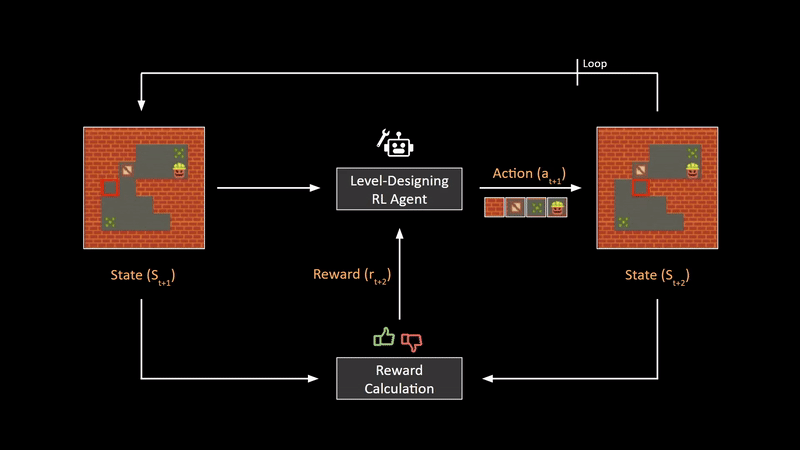
Reinforcement Learning
- designed for problems that involve decision-making in sequential action
- You have some sort of agent that “explores” some space
- As it goes, it learns the value of different state changes in different conditions
- Those values inform subsequent behavior of the agent
- Examples: Pac-Man, Cat & Mouse game (game AI)
- Supply chain management
- HVAC systems
- Industrial robotics
- Dialog systems
- Autonomous vehicles
- Yields fast on-line performance once the space has been explored
- Q-Learning
- A set of environmental states s
- A set of possible actions in those states a
- A value of each state/action Q
- Start off with Q values of 0
- Explore the space
- As bad things happen after a given state/action, reduce its Q
- As rewards happen after a given state/action, increase its Q
- can “look ahead” more than one step by using a discount factor when computing Q (here s is previous state, s’ is current state)
- Q(s,a) += discount * (reward(s,a) + max(Q(s’)) – Q(s,a))
- The exploration problem
- efficiently explore all of the possible states
- Simple approach: always choose the action for a given state with the highest Q. If there’s a tie, choose at random
- But that’s really inefficient, and you might miss a lot of paths that way
- Better way: introduce an epsilon term
- If a random number is less than epsilon, don’t follow the highest Q, but choose at random
- That way, exploration never totally stops
- Choosing epsilon can be tricky
- Markov Decision Process (MDP)
- modeling decision making in situations where outcomes are partly random and partly under the control of a decision maker
- States are still described as s and s’
- State transition functions are described as 𝑃𝑎 (𝑠, 𝑠′)
- Our “Q” values are described as a reward function 𝑅𝑎 (𝑠, 𝑠′)
- a discrete time stochastic control process.
- modeling decision making in situations where outcomes are partly random and partly under the control of a decision maker
- RL in SageMaker
- Uses a deep learning framework with Tensorflow and MXNet
- Supports Intel Coach and Ray Rllib toolkits.
- MATLAB, Simulink
- EnergyPlus, RoboSchool, PyBullet
- Amazon Sumerian, AWS RoboMaker
- Distributed Training with SageMaker RL
- Can distribute training and/or environment rollout
- Multi-core and multi-instance
- Key Terms
- Environment
- The layout of the board / maze / etc
- State
- Where the player / pieces are
- Action
- Move in a given direction, etc
- Reward
- Value associated with the action from that state
- Observation
- i.e., surroundings in a maze, state of chess board
- Environment
- Hyperparameters
- Parameters of your choosing may be abstracted
- Hyperparameter tuning in SageMaker can then optimize them
- Instance Types
- deep learning – so GPU’s are helpful
- supports multiple instances and cores