Data Types
- Numerical
- Represents some sort of quantitative measurement
- Discrete Data: Integer based; often counts of some event
- Continuous Data: Has an infinite number of possible values
- Categorical
- Qualitative data that has no inherent mathematical meaning
- You can assign numbers to categories in order to represent them more compactly, but the numbers don’t have mathematical meaning
- Ordinal
- A mixture of numerical and categorical
- Categorical data that has mathematical meaning
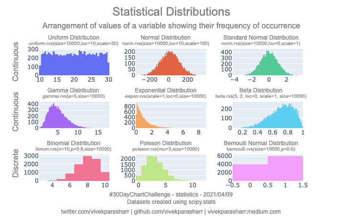
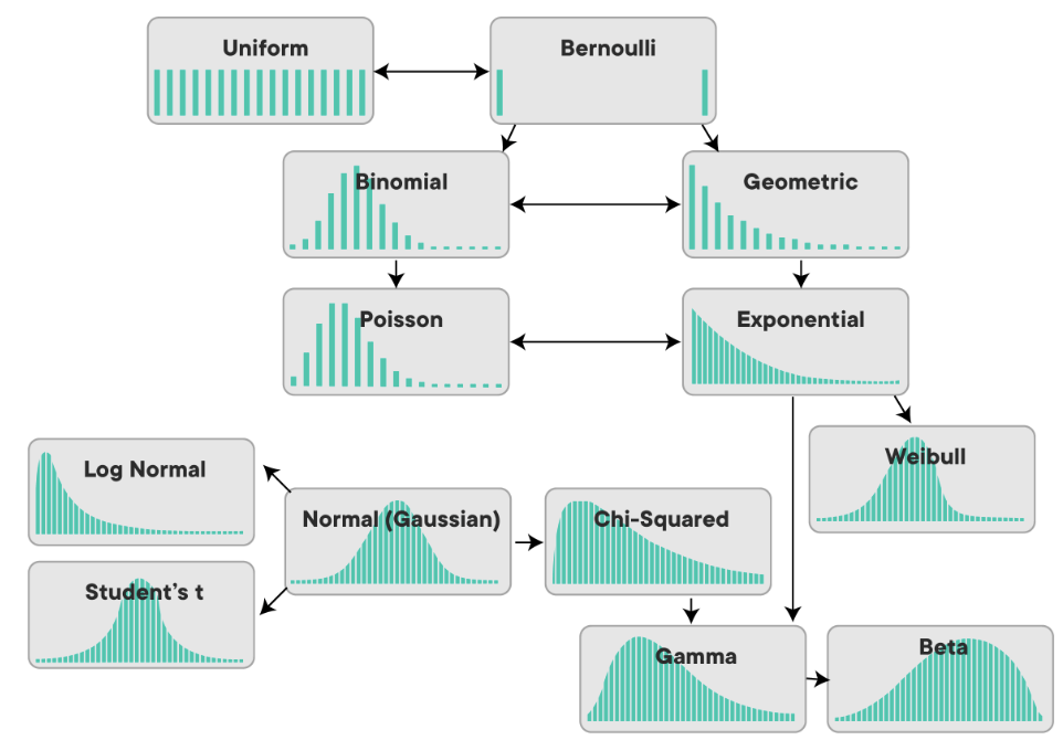
Data Distributions
- Normal distribution
- Probability Mass Function
- aka, probability function, frequency function, discrete probability density function
- a function that gives the probability that a discrete random variable is exactly equal to some value. The probability mass function is often the primary means of defining a discrete probability distribution, and such functions exist for either scalar or multivariate random variables whose domain is discrete.
- Poisson Distribution
- expresses the probability of a given number of events occurring in a fixed interval of time if these events occur with a known constant mean rate and independently of the time since the last event.
- A classic example used to motivate the Poisson distribution is the number of radioactive decay events during a fixed observation period.
- A Poisson distribution is a probability distribution that is used to show how many times an event is likely to occur over a specified period. In other words, it is a count distribution. Poisson distributions are often used to understand independent events that occur at a constant rate within a given interval of time.
- Binomial Distribution
- In probability theory and statistics, the binomial distribution with parameters n and p is the discrete probability distribution of the number of successes in a sequence of n independent experiments, each asking a yes–no question, and each with its own Boolean-valued outcome: success (with probability p) or failure (with probability q = 1 − p). A single success/failure experiment is also called a Bernoulli trial or Bernoulli experiment, and a sequence of outcomes is called a Bernoulli process; for a single trial, i.e., n = 1, the binomial distribution is a Bernoulli distribution.
- Bernoulli Distribution
- Special case of binomial distribution
- Has a single trial (n=1)
- Can think of a binomial distribution as the sum of Bernoulli distributions
Time Series Analysis
- Trends
- Seasonality
- Noise
- Seasonality + Trends + Noise = time series
- Additive model
- A data model in which the effects of individual factors are differentiated and added together to model the data.
- Seasonal variation is constant
- Additive model
- seasonality * trends * noise
- Multiplicative model
- assumes that as the data increase, so does the seasonal pattern. Most time series plots exhibit such a pattern
- Seasonal variation increases as the trend increases
- Multiplicative model
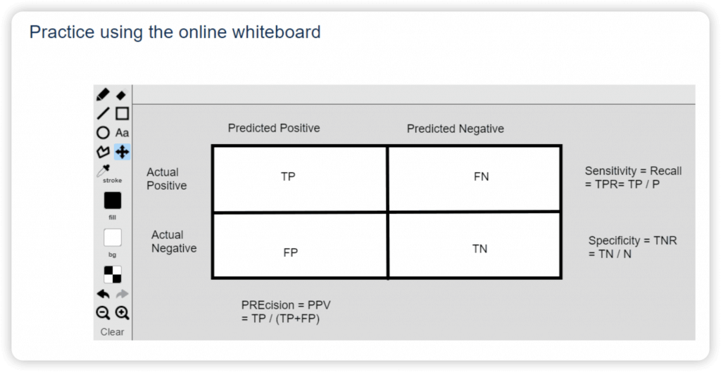
Confusion Matrix
| Predicted condition | |||
| Total population = P + N | Positive (PP) | Negative (PN) | |
| Actual condition | Positive (P) | True positive (TP) | False negative (FN) |
| Negative (N) | False positive (FP) | True negative (TN) | |
- aka Error Matrix, or matching matrix
- Each row of the matrix represents the instances in an actual class while each column represents the instances in a predicted class, or vice versa – both variants are found in the literature. The diagonal of the matrix therefore represents all instances that are correctly predicted.
- Total population = P + N
- True Positive Rate (TPR) = Recall = Sensitivity (SEN) = Hit Rate = Completeness = TP / P = TP / (TP + FN) = 1 – FNR
- how well the model identifies true positives
- Good choice of metric when you care a lot, about false negatives, i.e., fraud detection
- The higher, the better
- Raise TPR, usually it may bring higher FPR, so be careful.
- False Negative Rate (FNR) = Miss Rate = Type II Error = FN / P = 1 – TPR
- False Positive Rate (FPR) = Type I Error = FP / N = 1 – TNR
- The lower, the better
- True Negative Rate (TNR) = Specificity (SPC) = Selectivity = TN / N = 1 – FPR
- True Positive Rate (TPR) = Recall = Sensitivity (SEN) = Hit Rate = Completeness = TP / P = TP / (TP + FN) = 1 – FNR
- Prevalence = P / (P+N)
- Positive Predictive Value (PPV) = Precision = Correct Positives = TP / (TP + FP) = 1 – FDR
- the quality of positive predictions
- Good choice of metric when you care a lot, about false positives, i.e., medical screening, drug testing
- False Omission Rate (FOR) = FN / (TN + FN) = 1 – NPV
- Positive Predictive Value (PPV) = Precision = Correct Positives = TP / (TP + FP) = 1 – FDR
- Accuracy (ACC) = (TP + TN) / (P + N)
- False Discovery Rate (FDR) = FP / (TP + FP) = 1 – PPV
- Negative Predictive Value (NPV) = FN / (TN + FN) = 1 – FOR
- Balanced Accuracy (BA) = (TPR + TNR) / 2
- F-Score = ( (1+b2) * Precision x Recall ) / ( (b2) Precision + Recall )
- when b = 1, ie F1-Score = 2 (PPV x TPR / (PPV + TPR)) = 2TP / (2TP + FP + FN)
- The F1 Score provides a balanced measure of a model’s performance by considering both precision (true predicted positive in all predicted positive) and recall (true predicted positive in all true positive).
- when b = 1, ie F1-Score = 2 (PPV x TPR / (PPV + TPR)) = 2TP / (2TP + FP + FN)
- Threat Score (TS) = Critical Success Index (CSI) = TP / (TP + FN + FP)
- F-Score = ( (1+b2) * Precision x Recall ) / ( (b2) Precision + Recall )
- Root mean squared error (RMSE) is another Accuracy measurement
- measure the differences between predicted values and actual values in a regression problem
- the square root of the average squared differences between the predicted and actual values
- the lower, the better
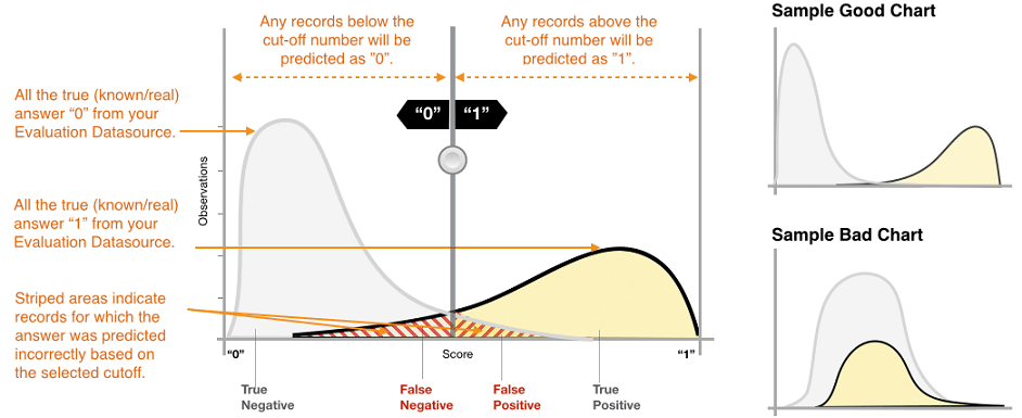
- Cut-off (or threshold) is a value used to convert the model’s predicted probabilities or scores into binary class predictions.
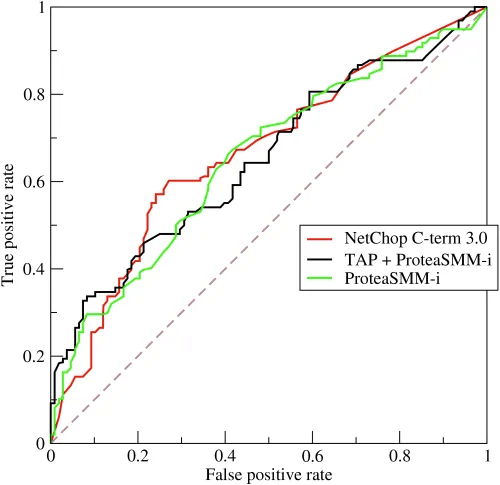
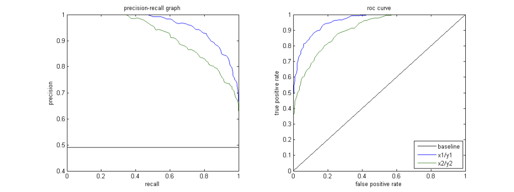
- Receiver Operating Characteristic Curve (ROC)
- Plot of true positive rate (recall) vs. false positive rate at various threshold settings
- Curve bent more on “upper-left” the better
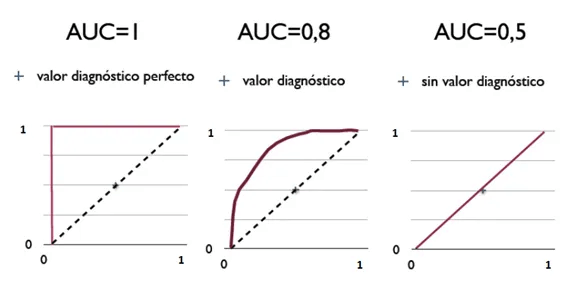
- Area Under the Curve (AUC)
- The area under the ROC curve
- probability that a classifier will rank a randomly chosen positive instance higher than a randomly chosen negative one
- ROC AUC of 0.5 is a useless classifier (Random), 1.0 is perfect
- To compare different classifiers, it can be useful to summarize the performance of each classifier into a single measure. One common approach is to calculate the area under the ROC curve (AUC.)
- AUC measures the ability of the model to predict a higher score for positive examples as compared to negative examples. Since AUC is independent of the selected threshold, you can get a sense of the prediction performance of your model from the AUC metric without picking a threshold.
- P-R Curve
- Precision / Recall curve
- Good = higher area (PR-AUC) under curve, ie more “upper-right” the better
- When to use
- Imbalanced Datasets: When the positive class is rare, and the dataset is heavily imbalanced, the PR curve is more informative than the ROC curve.
- Examples include fraud detection and disease diagnosis.
- Costly False Positives: If false positives are more costly or significant than false negatives, such as in spam email detection, the PR curve is more suitable as it focuses on precision.
- Imbalanced Datasets: When the positive class is rare, and the dataset is heavily imbalanced, the PR curve is more informative than the ROC curve.
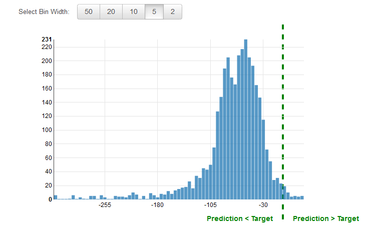
- A residual for an observation in the evaluation data is the difference between the true target and the predicted target. Residuals represent the portion of the target that the model is unable to predict. A positive residual indicates that the model is underestimating the target (the actual target is larger than the predicted target). A negative residual indicates an overestimation (the actual target is smaller than the predicted target).
- The histogram of the residuals on the evaluation data, when distributed in a bell shape and centered at zero, indicates that the model makes mistakes in a random manner and does not systematically over or under predict any particular range of target values. If the residuals do not form a zero-centered bell shape, there is some structure in the model’s prediction error.
| Data Type | Method | Note |
|---|---|---|
| Binary / Category | Recall / Sensitivity / True Positive Rate (in actual) | TP / (TP + FN) |
| True Negative Rate / Specificity / Selectivity | TN / (TN + FP) | |
| Precision (in prediction) | TP / (TP + FP) | |
| Accuracy | (TP + TN) / ((TP + FN) + (FP + TN)) | |
| False Negative Rate / Miss Rate | FN / (TP + FN) | |
| F1-Score | 2TP / (2TP + FP + FN) | |
| Root mean squared error (RMSE) | ||
| Area Under the Curve (AUC) | ||
| P-R Curve | Precision / Recall curve | |
| Log loss | a classification metric designed for models that output probabilities for class predictions | |
| Numeric | Residual | evaluating regression models; positive means under-estimate, and negative means over-estimate; so the visualization of Residual can give hint on the “overfit” or “underfit”, but not exact numeric value for models comparison. |
| Root mean squared error (RMSE) | standard metric for evaluating regression models (Accuracy); however, it cannot tell whether the model is overfit nor underfit | |
| Average Weighted Quantile Loss (Average wQL) | for probabilistic forecasting, where one predicts a range (distribution) of possible future values rather than a single point. It’s beneficial in time-series models like those used in weather forecasting, where uncertainty and quantiles matter |
Feature Engineering
- A feature is an individual measurable property within a recorded dataset. In machine learning and statistics, features are often called “variables” or “attributes.” Relevant features have a correlation or bearing (called feature importance) on a model’s use case.
- Applying your knowledge of the data – and the model you’re using – to create better features to train your model with.
- Which features should I use?
- Do I need to transform these features in some way?
- How do I handle missing data?
- Should I create new features from the existing ones?
- You can’t just throw in raw data and expect good results
- The Curse of Dimensionality
- Too many features can be a problem – leads to sparse data
- Every feature is a new dimension
- Much of feature engineering is selecting the features most relevant to the problem at hand
- This often is where domain knowledge comes into play
- Unsupervised dimensionality reduction techniques can also be employed to distill many features into fewer features
- Principal component analysis (PCA) is a linear dimensionality reduction technique with applications in exploratory data analysis, visualization and data preprocessing.
- K-Means aims to partition n observations into k clusters in which each observation belongs to the cluster with the nearest mean (cluster centers or cluster centroid), serving as a prototype of the cluster.
Imputing Missing Data / Imputation
- In multiple imputations approach, you need to generate missing values from the dataset many times. The individual datasets are then pooled together into the final imputed dataset, with the values chosen to replace the missing data being drawn from the combined results in some way.The multiple imputations approach breaks imputation process into three steps: imputation (multiple times), analysis (staging how the results should be combined), and pooling (integrating the results into the final imputed matrix).
- Mean Replacement
- Replace missing values with the mean value from the rest of the column (columns, not rows! A column represents a single feature; it only makes sense to take the mean from other samples of the same feature.)
- Fast & easy, won’t affect mean or sample size of overall data set
- Median may be a better choice than mean when outliers are present
- But it’s generally pretty terrible.
- Only works on column level, misses correlations between features
- Can’t use on categorical features (imputing with most frequent value can work in this case, though)
- Not very accurate
- Dropping
- Reduce the final data records
- Machine Learning
- KNN: Find K “nearest” (most similar) rows and average their values
- Assumes numerical data, not categorical
- Deep Learning
- Build a machine learning model to impute data for your machine learning model!
- Works well for categorical data. Really well. But it’s complicated.
- Regression
- Find linear or non-linear relationships between the missing feature and other features
- Most advanced technique: MICE (Multiple Imputation by Chained Equations)
- creating multiple imputed datasets by using chained equations, where each feature with missing data is modeled based on the other features in the dataset. MICE iteratively imputes missing values, making the process more robust and ensuring that relationships among features are preserved. It’s particularly effective when dealing with complex datasets, where simple imputation methods, such as mean or median, might lead to biased results.
- KNN: Find K “nearest” (most similar) rows and average their values
Unbalanced Data
- Large discrepancy between “positive” and “negative” cases
- “positive” means the thing you’re testing for is what happened
- i.e., fraud detection. Fraud is rare, and most rows will be not-fraud
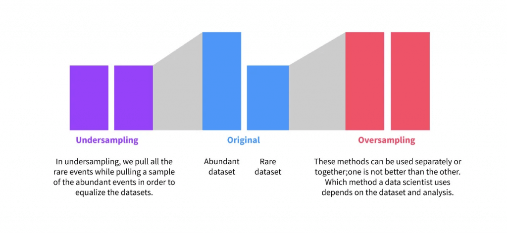
- Techniques for re-balance
- Oversampling
- Duplicate samples from the minority class
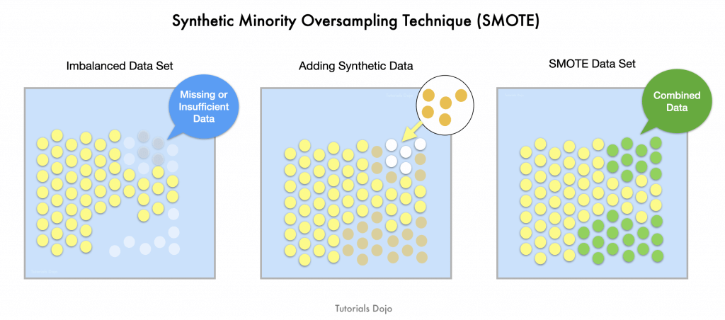
- Synthetic Minority Over-sampling TEchnique (SMOTE)
- The Synthetic Minority Oversampling Technique (SMOTE) is a popular technique for addressing class imbalance in machine learning. When the dataset has significantly fewer examples of a certain class, SMOTE generates synthetic examples to balance the dataset. Instead of simply duplicating existing minority class data points, SMOTE creates new, synthetic instances by interpolating between existing ones. This process helps to increase the variety and quantity of the minority class, which can improve the model’s ability to learn and detect patterns in that class, such as fraud, and reduce bias toward the majority class.
- SMOTE is beneficial in scenarios where the minority class is underrepresented, such as fraud detection, disease prediction, or rare event prediction. By ensuring the model gets a more balanced view of both classes, SMOTE enables better generalization and performance. It can be particularly useful when working with algorithms that struggle with class imbalance, such as decision trees, random forests, and neural networks. Implementing SMOTE generally leads to models that are more robust and effective at identifying rare events or behaviors in the data.
- This technique can be implemented through various machine learning libraries, such as
imblearnin Python, and is often used in conjunction with other techniques, like cross-validation and hyperparameter tuning, to ensure that the model performs well on both classes. It’s a valuable tool for handling class imbalance and improving the overall model performance in real-world applications like fraud detection
- Artificially generate new samples of the minority class using nearest neighbors
- Run K-nearest-neighbors of each sample of the minority class
- Create a new sample from the KNN result (mean of the neighbors)
- Both generates new samples and undersamples majority class
- Generally better than just simple oversampling
- Undersampling
- Instead of creating more positive samples, remove “some” negative ones
- Throwing data away is usually not the right answer
- Oversampling
- Adjusting thresholds
- When making predictions about a classification (fraud / not fraud), you have some sort of threshold of probability at which point you’ll flag something as the positive case (fraud)
- If you have too many false positives, one way to fix that is to simply increase that threshold.
- Guaranteed to reduce false positives
- But, could result in more false negatives

Outliers
- Variance (𝜎 2 ) is simply the average of the squared differences from the mean
- measures how “spread-out” the data is
- Standard Deviation 𝜎 is just the square root of the variance.
- Data points lie than one standard deviation from the mean can be considered unusual.
- how extreme a data point is by talking about “how many sigmas” away from the mean it is.
- Dealing with Outliers
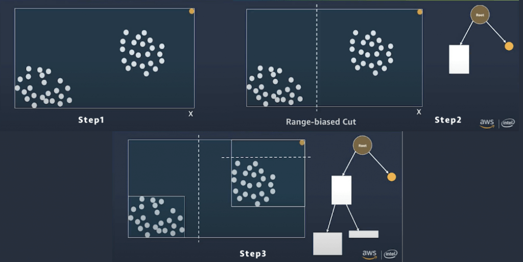
- AWS’s Random Cut Forest algorithm creeps into many of its services – it is made for outlier detection
- It takes a set of random data points, cuts them down to the same number of points, and then builds a collection of models. In contrast, a model corresponds to a decision tree—thus the name forest.
Binning / Bucketing
- Bucket observations together based on ranges of values.
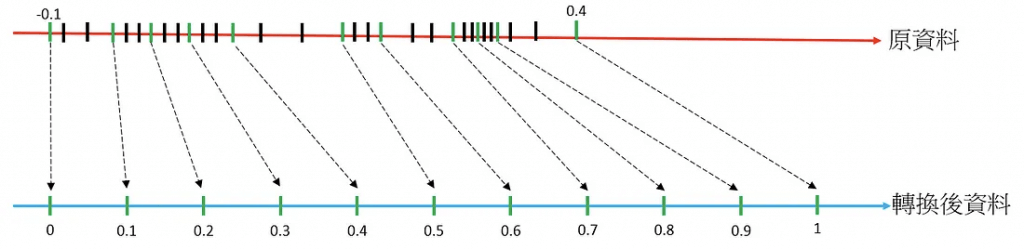
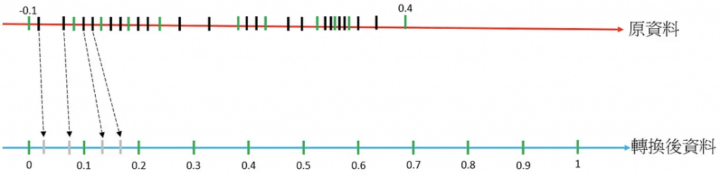
- Quantile binning categorizes data by their place in the data distribution
- Ensures even sizes of bins
- Transforms numeric data to categorical/ordinal data
- Especially useful when there is uncertainty in the measurements
Transforming
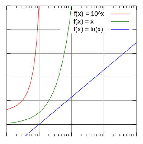
- A skewed distribution is bad for many models that is why we have to perform transformations on certain features to bring them as close to a normal distribution as possible.
- A positively skewed distribution contains values that mostly cluster to the left and has a longer right tail
- Logarithmic transformation
- Negative skewed distribution (that slow start from little for a while, the mostly cluster on the right)
- Third-order polynomial transformation
- Feature data with an exponential trend may benefit from a logarithmic transform
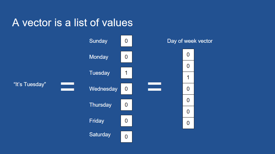
Encoding
- Transforming data into some new representation required by the model
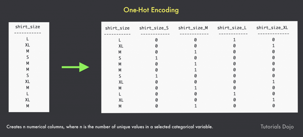
- One-Hot encoding
- Create “buckets” for every category
- These numerical values are binary digits composed of 0 and 1. It creates a number (n) of numerical columns, where n is the number of unique values in a selected categorical variable
- The bucket for your category has a 1, all others have a 0
- Very common in deep learning, where categories are represented by individual output “neurons”
| Decimal | Binary | Unary | One-hot |
|---|---|---|---|
| 0 | 000 | 00000000 | 00000001 |
| 1 | 001 | 00000001 | 00000010 |
| 2 | 010 | 00000011 | 00000100 |
| 3 | 011 | 00000111 | 00001000 |
| 4 | 100 | 00001111 | 00010000 |
| 5 | 101 | 00011111 | 00100000 |
| 6 | 110 | 00111111 | 01000000 |
| 7 | 111 | 01111111 | 10000000 |
Scaling / Normalization
- Some models prefer feature data to be normally distributed around 0 (most neural nets)
- Most models require feature data to at least be scaled to comparable values
- Otherwise features with larger magnitudes will have more weight than they should
- Example: modeling age and income as features – incomes will be much higher values than ages
- Remember to scale your results back up
Shuffling
- Many algorithms benefit from shuffling their training data
- Otherwise they may learn from residual signals in the training data resulting from the order in which they were collected
- The error of an observation is the deviation of the observed value from the true value of a quantity of interest (for example, a population mean). The residual is the difference between the observed value and the estimated value of the quantity of interest (for example, a sample mean).
Term Frequency and Inverse Document Frequency (TF-IDF)
- figures out what terms are most relevant for a document
- Term Frequency just measures how often a word occurs in a document
- A word that occurs frequently is probably important to that document’s meaning
- Document Frequency is how often a word occurs in an entire set of documents, i.e., all of Wikipedia or every web page
- This tells us about common words that just appear everywhere no matter what the topic, like “a”, “the”, “and”, etc.
- So a measure of the relevancy of a word to a document might be: 𝑇𝑒𝑟𝑚 𝐹𝑟𝑒𝑞𝑢𝑒𝑛𝑐𝑦 / 𝐷𝑜𝑐𝑢𝑚𝑒𝑛𝑡 𝐹𝑟𝑒𝑞𝑢𝑒𝑛𝑐𝑦, (aka Term Frequency * Inverse Document Frequency )
- That is, take how often the word appears in a document, over how often it just appears everywhere. That gives you a measure of how important and unique this word is for this document
- In practice, the TF-IDF often use TF * Inverse (log of) Document Frequency, since word frequencies are distributed exponentially.
- n-gram
- An n-gram is a sequence of n adjacent symbols in particular order. The symbols may be n adjacent letters (including punctuation marks and blanks), syllables, or rarely whole words found in a language dataset; or adjacent phonemes extracted from a speech-recording dataset, or adjacent base pairs extracted from a genome.
- Unigrams: single word
- Bi-grams: two close-by terms
- Tri-grams: three sequenced terms
- Example:
- The TF-IDF Matrix for unigram and bigrams of these two sentences
- Please call the number below.
- Please do not call us.
- the matrix dimension would be (2, 16)
- 2 – two input source (documents)
- 16 – 8 unigrams (“please”, “call”, “the”, “number”, “below”, “do”, “not”, “us”) + 8 bigrams (“please call”, “call the”, “the number”, “number below”, “please do”, “do not”, “not call”, “call us”)
- The TF-IDF Matrix for unigram and bigrams of these two sentences

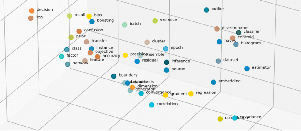
Embeddings
- Embeddings are numerical representations of real-world objects that machine learning (ML) and artificial intelligence (AI) systems use to understand complex knowledge domains like humans do.
- As an example, computing algorithms understand that the difference between 2 and 3 is 1, indicating a close relationship between 2 and 3 as compared to 2 and 100.
- However, real-world data includes more complex relationships. For example, a bird-nest and a lion-den are analogous pairs, while day-night are opposite terms.
- Embeddings convert real-world objects into complex mathematical representations that capture inherent properties and relationships between real-world data.
- Benefits
- Reduce data dimensionality
- Train large language models
- Build innovative applications
- relevant models/algorithms
- Principal component analysis
- Singular value decomposition
- Word2Vec / Object2Vec
- BERT

Model Evaluation
- Binary Model Insights
- Metrics
- Accuracy (ACC): (TP + TN) / (P + N), to maximize the ratio of correct predictions to total predictions
- Precision: TP / (TP + FP), to minimize false positives
- Recall: TP / (TP + FN), to minimize false negatives
- False Positive Rate (FPR): FP / (FP + TN)
- Area Under the (Receiver Operating Characteristic) Curve (AUC)
- measures the ability of the model to predict a higher score for positive examples as compared to negative examples
- a tradeoff between false positives and false negatives
- The actual output of many binary classification algorithms is a prediction score. The score indicates the system’s certainty that the given observation belongs to the positive class. To make the decision about whether the observation should be classified as positive or negative, as a consumer of this score, you will interpret the score by picking a classification threshold (cut-off) and compare the score against it. Any observations with scores higher than the threshold are then predicted as the positive class and scores lower than the threshold are predicted as the negative class.
- For the given use-case, the classification model predicts if a customer is likely to churn. This implies that a False Negative is very costly for the company because the model predicted that the customer will not churn, however, in reality the customer did churn. So the ideal model would focus on reducing the False Negatives.
- Metrics
- Multiclass Model Insights
- Metrics
- F1 Score: 2TP / (2TP + FP + FN)
- Metrics
- Regression Model Insights
- Metrics
- standard root mean square error (RMSE)
- Metrics
- Cross-Validation
- training several ML models on subsets of the available input data and evaluating them on the complementary subset of the data
- Good to check out the “overfitting”
- Cross-validation is a technique for evaluating ML models by training several ML models on subsets of the available input data and evaluating them on the complementary subset of the data. Use cross-validation to detect overfitting, i.e. failing to generalize a pattern.
In k-fold cross-validation, you split the input data into k subsets of data (also known as folds). You train your models on all but one (k-1) of the subsets and then evaluate them on the subset that was not used for training. This process is repeated k times, with a different subset reserved for evaluation (and excluded from training) each time.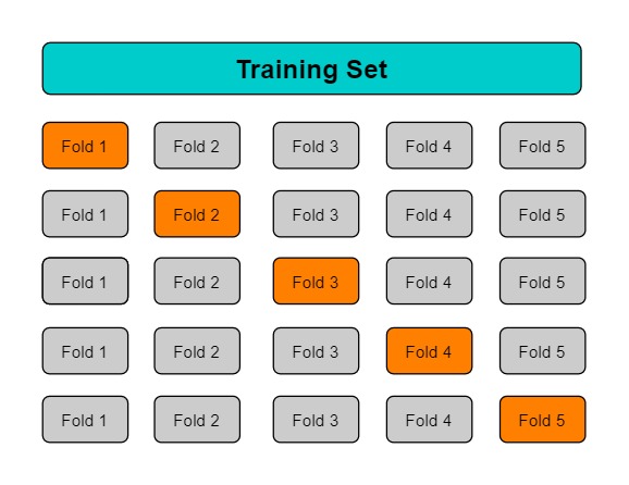
The diagram above shows an example of the training subsets and complimentary evaluation subsets generated for each of the four models that are created and trained during 4-fold cross-validation. Model one uses the first 25 percent of data for evaluation, and the remaining 75 percent for training. Model two uses the second subset of 25 percent (25 percent to 50 percent) for evaluation, and the remaining three subsets of the data for training, and so on.
Performing 4-fold cross-validation generates four models, four data sources to train the models, four data sources to evaluate the models, and four evaluations, one for each model. Amazon ML generates a model performance metric for each evaluation. For example, in 4-fold cross-validation for a binary classification problem, each of the evaluations reports an area under curve (AUC) metric. You can get the overall performance measure by computing the average of the four AUC metrics. - Evaluate each model performance through a confusion matrix is incorrect because this will just provide a visualization of how the model performed. It won’t generate a “score” that will serve as a useful metric to compare model performance.

AI inference vs. training
- Training is the first phase for an AI model. Training may involve a process of trial and error, or a process of showing the model examples of the desired inputs and outputs, or both.
- Inference is the process that follows AI training. The better trained a model is, and the more fine-tuned it is, the better its inferences will be — although they are never guaranteed to be perfect.
- The core of reasoning/inference is to apply a trained AI model to new data and make decisions based on the model’s predictions.
Data Transformations
- Normalization of numeric variables can help the learning process if there are very large range differences between numeric variables because variables with the highest magnitude could dominate the ML model, no matter if the feature is informative with respect to the target or not.
- Quantile Binning Transformation is incorrect. This is just a process used to discover non-linearity in the variable’s distribution by grouping observed values together. It won’t help normalize features with wide-ranging differences.
- The quantile binning processor takes two inputs, a numerical variable and a parameter called bin number, and outputs a categorical variable. The purpose is to discover non-linearity in the variable’s distribution by grouping observed values together.
- In many cases, the relationship between a numeric variable and the target is not linear (the numeric variable value does not increase or decrease monotonically with the target). In such cases, it might be useful to bin the numeric feature into a categorical feature representing different ranges of the numeric feature. Each categorical feature value (bin) can then be modeled as having its own linear relationship with the target. For example, let’s say you know that the continuous numeric feature account_age is not linearly correlated with likelihood to purchase a book. You can bin age into categorical features that might be able to capture the relationship with the target more accurately.
- N-gram Transformation is incorrect as this is simply used for splitting sentences into a list of word/s.
- The n-gram transformation takes a text variable as input and produces strings corresponding to sliding a window of (user-configurable) n words, generating outputs in the process.
- Orthogonal Sparse Bigram (OSB) Transformation is incorrect. Just like the N-gram Transformation, this transformation is intended to aid in text string analysis and is just an alternative to the bi-gram transformation.
- The OSB transformation is intended to aid in text string analysis and is an alternative to the bi-gram transformation (n-gram with window size 2). OSBs are generated by sliding the window of size n over the text, and outputting every pair of words that includes the first word in the window.
- “The quick brown fox”, {The_quick, The__brown, The___fox}
- “quick brown fox jumps”, {quick_brown, quick__fox, quick___jumps}
- “brown fox jumps over”, {brown_fox, brown__jumps, brown___over}
- “fox jumps over the”, {fox_jumps, fox__over, fox___the}
- “jumps over the lazy”, {jumps_over, jumps__the, jumps___lazy}
- “over the lazy dog”, {over_the, over__lazy, over___dog}
- “the lazy dog”, {the_lazy, the__dog}
- “lazy dog”, {lazy_dog}
- The OSB transformation is intended to aid in text string analysis and is an alternative to the bi-gram transformation (n-gram with window size 2). OSBs are generated by sliding the window of size n over the text, and outputting every pair of words that includes the first word in the window.
- Cartesian Product Transformation
- The Cartesian transformation generates permutations of two or more text or categorical input variables. This transformation is used when an interaction between variables is suspected. For example, consider the bank marketing dataset that is used in Tutorial: Using Amazon ML to Predict Responses to a Marketing Offer. Using this dataset, we would like to predict whether a person would respond positively to a bank promotion, based on the economic and demographic information. We might suspect that the person’s job type is somewhat important (perhaps there is a correlation between being employed in certain fields and having the money available), and the highest level of education attained is also important. We might also have a deeper intuition that there is a strong signal in the interaction of these two variables—for example, that the promotion is particularly well-suited to customers who are entrepreneurs who earned a university degree.
- The Cartesian product transformation takes categorical variables or text as input, and produces new features that capture the interaction between these input variables.
- Tokenization is incorrect because this method is commonly used in Natural Language Processing (NLP) where you split a string into a list of words that have a semantic meaning.
It may reduce the overall size of the dataset, but it won’t help at all in reducing highly correlated features. In Linear Algebra, matrix multiplication is a binary operation that produces a matrix from two matrices or in other words, it multiplies two matrices that are usually in array form. In Machine Learning, matrix multiplication is a compute-intensive operation used to process sparse or scattered data produced by the training model.
A Bayesian network is a representation of a joint probability distribution of a set of random variables with a possible mutual causal relationship. The network consists of nodes representing the random variables, edges between pairs of nodes representing the causal relationship of these nodes, and a conditional probability distribution in each of the nodes.
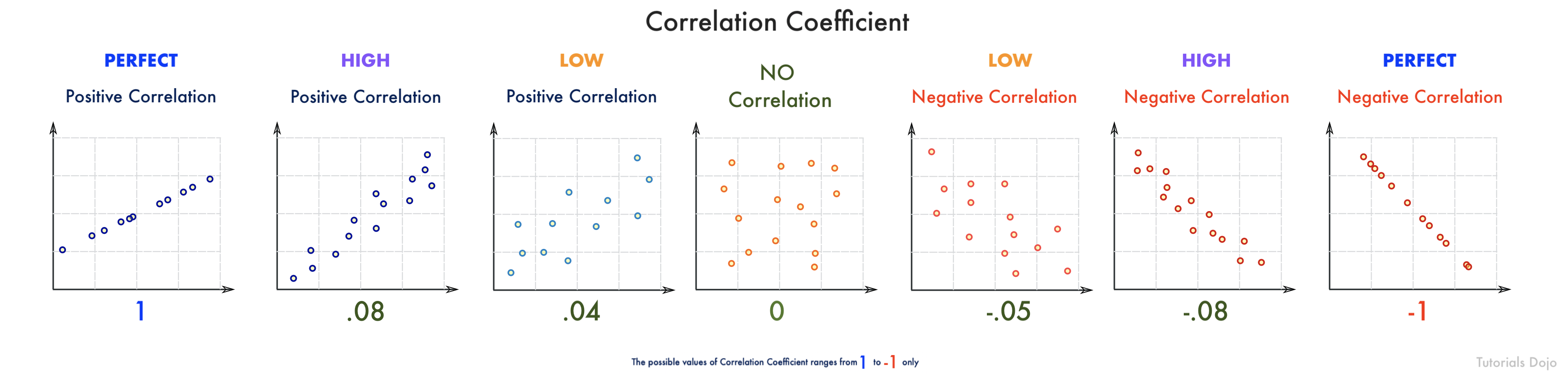
The Pearson’s correlation coefficient measures the statistical relationship between two variables. A correlation coefficient that is closer to 1 means that there’s a positive correlation between two variables (X increases as Y increases), while a correlation coefficient closer to -1 suggests a negative correlation (X increases as Y decreases). As the correlation coefficient approaches 0, the weaker the correlation between the measured variables gets.
In this scenario, A full Bayesian network will be more performant than a Naive Bayesian since there are varying dependencies between each variable (0.1 – 0.97).
The performance of a Naive Bayesian model heavily relies on how strongly independent the predictors are. Since there are some highly correlated predictors in the dataset, a Full Bayesian network is more suitable.