== GENERAL / TABULAR ==
Linear Learner
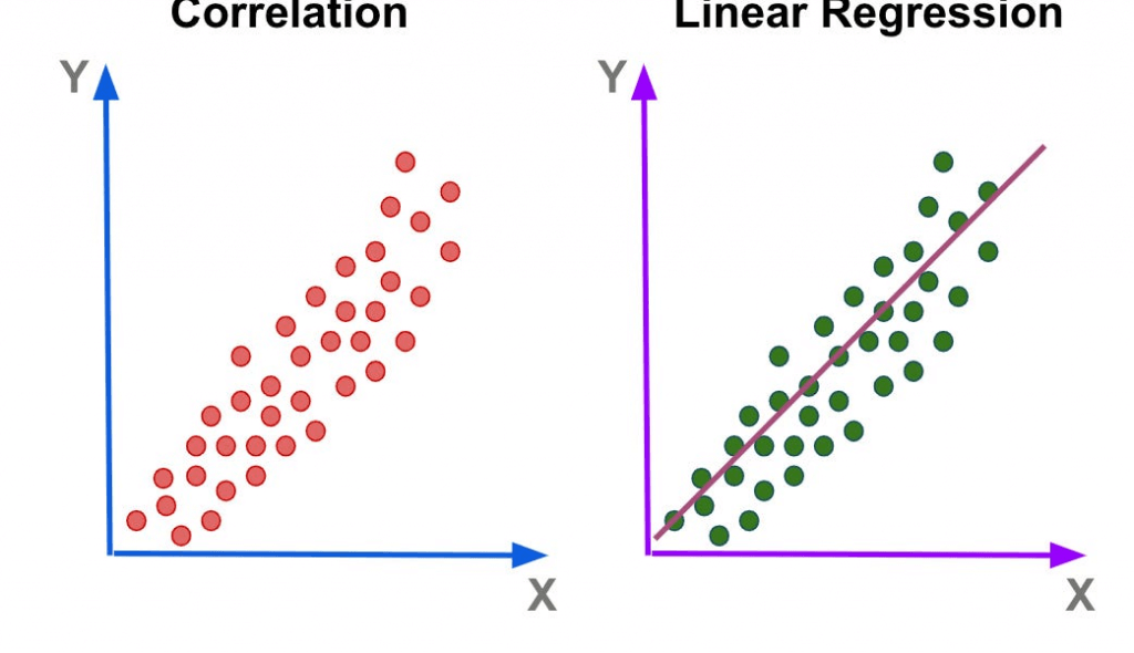
- Linear regression
- Logistic regression produces a binary output
- Main Use Cases
- regression (numeric) predictions
- classification predictions
- Inputs
- RecordIO-wrapped protobuf
- Float32 data only!
- CSV
- First column assumed to be the label
- File or Pipe mode both supported
- RecordIO-wrapped protobuf
- Processes
- Preprocessing
- Training data must be normalized (so all features are weighted the same)
- Input data should be shuffled
- Training
- Uses stochastic gradient descent
- Choose an optimization algorithm (Adam, AdaGrad, SGD, etc)
- Multiple models are optimized in parallel
- Tune L1, L2 regularization
- Validation
- Most optimal model is selected
- Preprocessing
- Hyperparameters
- Balance_multiclass_weights
- Gives each class equal importance in loss functions
- Learning_rate, mini_batch_size
- L1 : Regularization
- Wd : Weight decay (L2 regularization)
- target_precision
- Use with binary_classifier_model_selection_criteria set to
recall_at_target_precision - Holds precision at this value while maximizing recall
- Use with binary_classifier_model_selection_criteria set to
- target_recall
- Use with binary_classifier_model_selection_criteria set to
precision_at_target_recall - Holds recall at this value while maximizing precision
- Use with binary_classifier_model_selection_criteria set to
- Balance_multiclass_weights
- Instance Types
- multi-GPU models not suitable
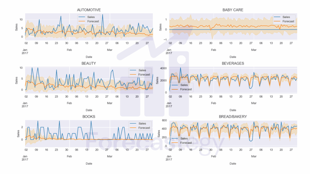
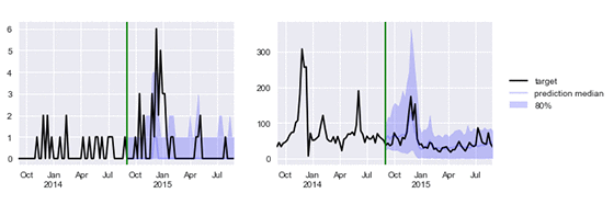
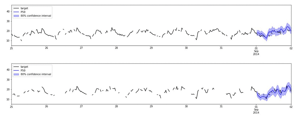
DeepAR Forecast
- Forecasting one-dimensional time series data
- Uses RNN’s
- Allows you to train the same model over several related time series
- Main Use Cases
- Finds frequencies and seasonality
- Input
- JSON (Gzip or Parquet)
- Each record must contain:
- Start: the starting time stamp
- Target: the time series values
- Optional
- Dynamic_feat: dynamic features (such as, was a promotion applied to a product in a time series of product purchases)
- Cat: categorical features
- Hyperparameters
- Context_length
- Number of time points the model sees before making a prediction
- Can be smaller than seasonalities; the model will lag one year anyhow.
- Epochs
- mini_batch_size
- Learning_rate
- Num_cells
- Context_length
- Instance Types
- CPU, GPU, single or multiple, all good
- GPU better for larger models, or with large mini-batch sizes (>512)
- CPU-only for reference
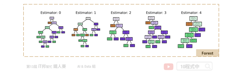
Random (Cut) Forest
- Anomaly detection
- Unsupervised
- Detect unexpected spikes in time series data
- Breaks in periodicity
- Unclassifiable data points
- Assigns an anomaly score to each data point
- Input
- RecordIO-protobuf or CSV
- Can use File or Pipe mode on either
- Optional test channel for computing accuracy, precision, recall, and F1 on labeled data (anomaly or not)
- Processing
- Creates a forest of trees where each tree is a partition of the training data; looks at expected change in complexity of the tree as a result of adding a point into it
- Data is sampled randomly
- Then trained
- RCF shows up in Kinesis Analytics as well; it can work on streaming data too.
- Hyperparameters
- Num_trees
- Increasing reduces noise
- Num_samples_per_tree
- Should be chosen such that 1/num_samples_per_tree approximates the ratio of anomalous to normal data
- Num_trees
- Instance Types
- Does not take advantage of GPUs
IP Insights
- Unsupervised learning of IP address usage patterns
- Main Use Cases
- Identifies suspicious behavior from IP addresses
- Identify logins from anomalous IP’s
- Identify accounts creating resources from anomalous IP’s
- Identifies suspicious behavior from IP addresses
- Input
- User names, account ID’s can be fed in directly; no need to pre-process
- Training channel, optional validation (computes AUC score)
- CSV only
- Entity, IP
- Processing
- Uses a neural network to learn latent vector representations of entities and IP addresses.
- Entities are hashed and embedded
- Need sufficiently large hash size
- Automatically generates negative samples during training by randomly pairing entities and IP’s
- Hyperparameters
- Num_entity_vectors
- Hash size
- Set to twice the number of unique entity identifiers
- Vector_dim
- Size of embedding vectors
- Scales model size
- Too large results in overfitting
- Epochs, learning rate, batch size, etc.
- Num_entity_vectors
- Instance Types
- CPU or GPU
- GPU recommended
- Can use multiple GPU’s
- Size of CPU instance depends on vector_dim and num_entity_vectors
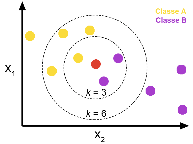
K-Nearest-Neighbors (KNN)
- Classification
- Find the K closest points to a sample point and return the most frequent label
- Regression
- Find the K closest points to a sample point and return the average value
- Input
- Train channel contains your data
- Test channel emits accuracy or MSE
- recordIO-protobuf or CSV training
- First column is label
- File or pipe mode on either
- Processing
- Data is first sampled
- SageMaker includes a dimensionality reduction stage
- Avoid sparse data (“curse of dimensionality”)
- At cost of noise / accuracy
- “sign” or “fjlt” methods
- Build an index for looking up neighbors
- Serialize the model
- Query the model for a given K
- Hyperparameters
- K!
- Sample_size
- Instance Types
- Training on CPU or GPU
- Inference
- CPU for lower latency
- GPU for higher throughput on large batches
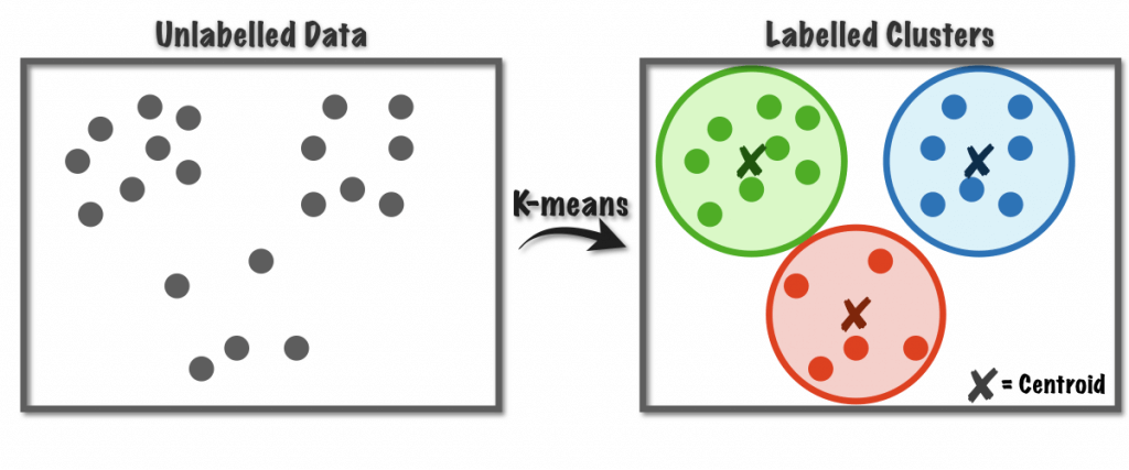
K-Means
- Unsupervised clustering
- Divide data into K groups, where members of a group are as similar as possible to each other
- You define what “similar” means
- Measured by Euclidean distance
- Input
- Train channel, optional test
- Train ShardedByS3Key, test FullyReplicated
- recordIO-protobuf or CSV
- File or Pipe on either
- Train channel, optional test
- Processing
- Every observation mapped to n-dimensional space (n = number of features)
- Works to optimize the center of K clusters
- “extra cluster centers” may be specified to improve accuracy (which end up getting reduced to k)
- K = k*x
- Algorithm:
- Determine initial cluster centers
- Random or k-means++ approach
- K-means++ tries to make initial clusters far apart
- Iterate over training data and calculate cluster centers
- Reduce clusters from K to k
- Using Lloyd’s method with kmeans++
- Determine initial cluster centers
- Hyperparameters
- K!
- Choosing K is tricky
- Plot within-cluster sum of squares as function of K
- Use “elbow method”
- Basically optimize for tightness of clusters
- Mini_batch_size
- Extra_center_factor
- Init_method
- K!
- Instance Types
- CPU or GPU, but CPU recommended
- Only one GPU per instance used on GPU
- CPU or GPU, but CPU recommended
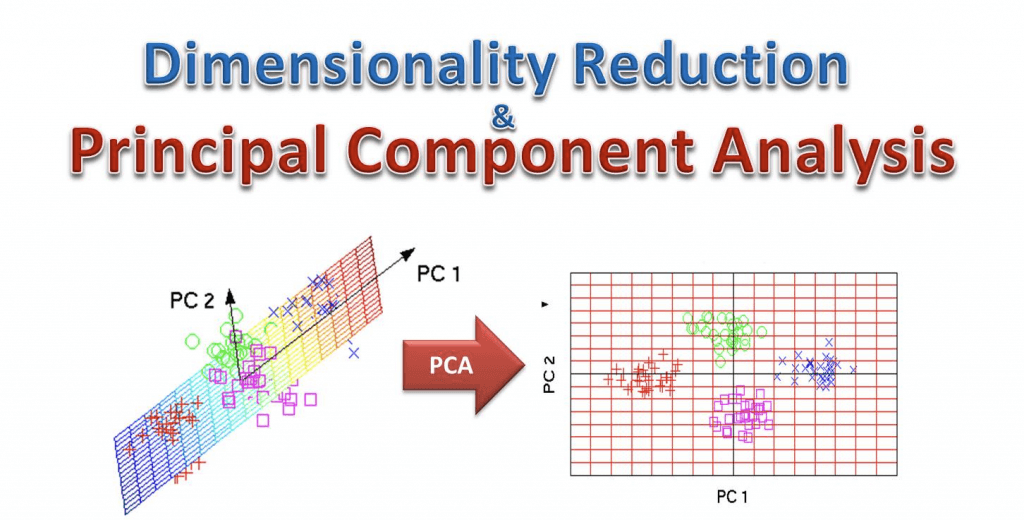
Principal Component Analysis (PCA)
- Dimensionality reduction
- Project higher-dimensional data (lots of features) into lower-dimensional (like a 2D plot) while minimizing loss of information
- The way PCA reduces the dimension is based on correlations.
- The reduced dimensions are called components
- First component has largest possible
variability - Second component has the next largest…
- First component has largest possible
- commonly used for feature extraction or visualization
- Unsupervised
- Input
- recordIO-protobuf or CSV
- File or Pipe on either
- Processing
- Covariance matrix is created, then singular value decomposition (SVD)
- Two modes
- Regular, for sparse data and moderate number of observations and features
- Randomized, for large number of observations and features
- Uses approximation algorithm
- Hyperparameters
- Algorithm_mode
- Subtract_mean
- Unbias data
- Instance Types
- GPU or CPU
- It depends “on the specifics of the input data”
- GPU or CPU
The t-Distributed Stochastic Neighbor Embedding (TSNE) is a non-linear dimensionality reduction algorithm used for exploring high-dimensional data. PCA and t-SNE are both valid dimensionality reduction techniques that you can use.
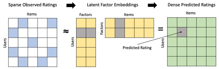
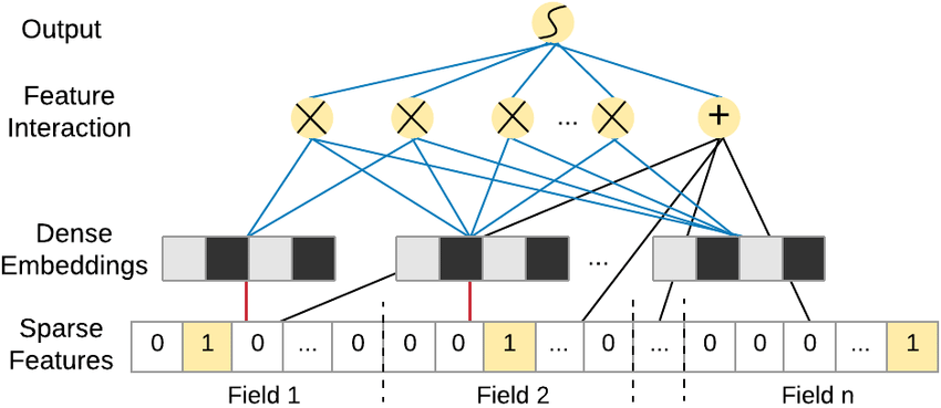
Factorization Machines ???
- Dealing with high dimensional sparse data
- Click prediction
- Item recommendations
- Since an individual user doesn’t interact with most pages / products the data is sparse
- Supervised
- Classification or regression
- Limited to pair-wise interactions
- User -> item for example
- Finds factors we can use to predict a classification (click or not? Purchase or not?) or value (predicted rating?) given a matrix representing some pair of things (users & items?)
- Usually used in the context of recommender systems
- Input
- recordIO-protobuf with Float32
- Sparse data means CSV isn’t practical
- recordIO-protobuf with Float32
- Hyperparameters
- Initialization methods for bias, factors, and linear terms
- Uniform, normal, or constant
- Can tune properties of each method
- Initialization methods for bias, factors, and linear terms
- Instance Types
- CPU or GPU
- CPU recommended
- GPU only works with dense data
- CPU or GPU

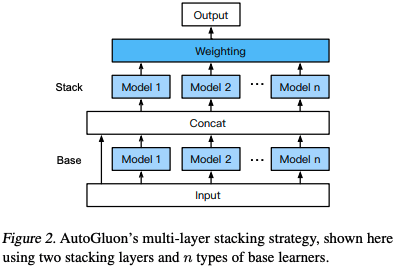
AutoGluon-Tabular
- an open-source AutoML framework that succeeds by ensembling models and stacking them in multiple layers
- Main Use Cases
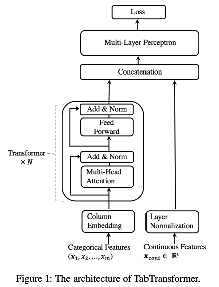
- use TabTransformer for regression, classification (binary and multiclass), and ranking problems
- Inputs
- CSV
- the rows representing observations, one column representing the target variable or label, and the remaining columns representing features.
- CSV
- Processes
- automatically recognizes the data type in each column for robust data preprocessing, including special handling of text fields
- models are stacked in multiple layers and trained in a layer-wise manner that guarantees raw data can be translated into high-quality predictions within a given time constraint
- Hyperparameters
- xxxxxxx
- Instance Types
- only train on a single machine (CPU or GPU, no multi-GPU)
TabTransformer
- built on self-attention-based Transformers
- Main Use Cases
- xxxxxxx
- Inputs
- CSV
- Processes
- xxxxxx
- Hyperparameters
- xxxxxxx
- Instance Types
- only train on a single machine (CPU or GPU, no multi-GPU)
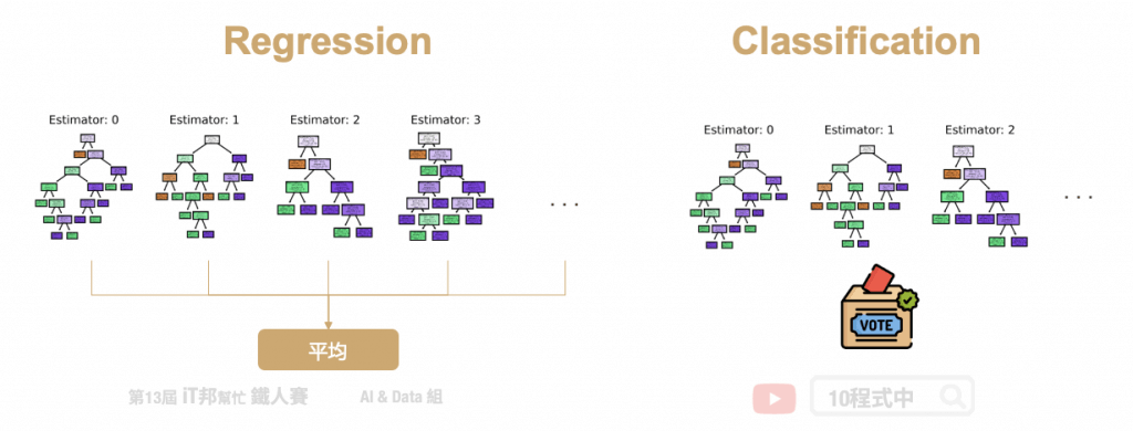
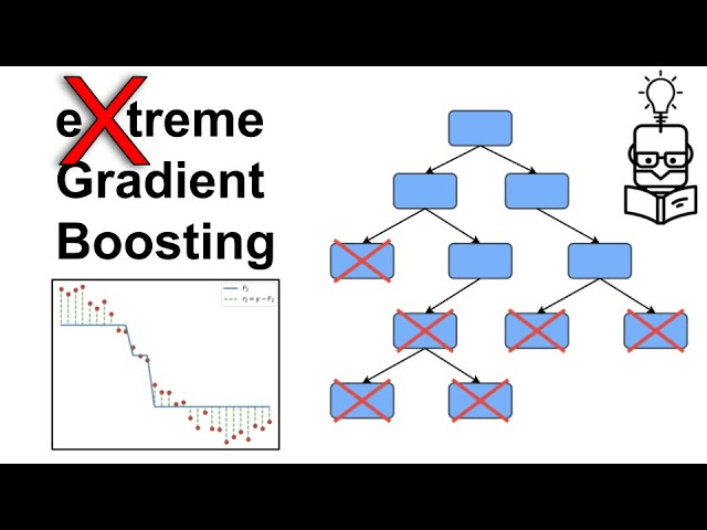
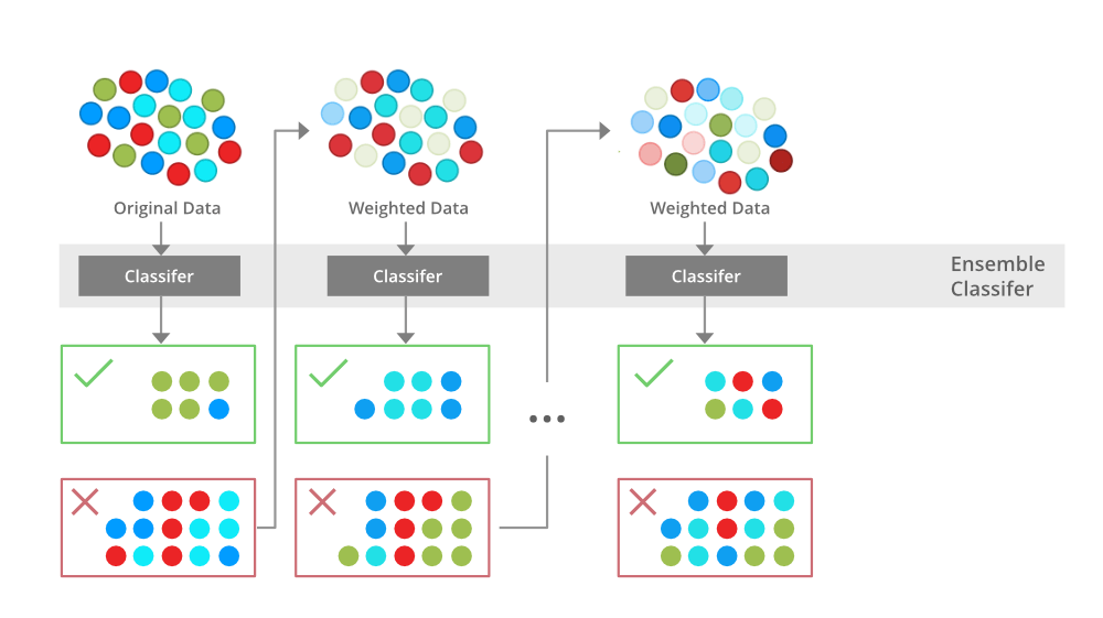
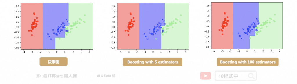
XGBoost
- use Gradient Boosting Decision Tree (GBDT) algorithm
- eXtreme Gradient Boosting
- Boosted group of decision trees
- New trees made to correct the errors of previous trees
- Uses gradient descent to minimize loss as new trees are added
- Main Use Cases
- classification ((binary and multiclass)
- regression, using regression trees
- ranking problems
- including financial forecasting, credit scoring, and customer churn prediction
- Inputs
- RecordIO-protobuf
- CSV
- libsvm
- Parquet
- Hyperparameters
- Subsample
- Prevents overfitting
- Eta
- Step size shrinkage, prevents overfitting
- Gamma
- Minimum loss reduction to create a partition; larger = more conservative
- Alpha
- L1 regularization term; larger = more conservative
- Lambda
- L2 regularization term; larger = more conservative
- eval_metric
- Optimize on AUC, error, rmse…
- For example, if you care about false positives more than accuracy, you might use AUC here
- MAP (Mean Average Precision) works only in evaluating ranking algorithms
- scale_pos_weight
- Adjusts balance of positive and negative weights
- Helpful for unbalanced classes
- Might set to sum(negative cases) / sum(positive cases)
- max_depth
- Max depth of the tree
- Too high and you may overfit
- Subsample
- Instance Types
- Is memory-bound, not compute-bound
- So, M5 is a good choice
- XGBoost 1.2
- single-instance GPU training is available
- Must set tree_method hyperparameter to gpu_hist
- XGBoost 1.5+: Distributed GPU training
- Must set use_dask_gpu_training to true
- Set distribution to fully_replicated in TrainingInput
- Only works with csv or parquet input
- Tuning Metrix
- Regression
- Root Mean Square Error (RMSE) “validation: rmse”
- Mean Absolute Error (MAE) “validation: mae”
- (Binary) Classification
- F1 is best, as combination of precision and recall, especially for imbalanced dataset “validation: f1”
- then Error “validation: error” or Accuracy “validation: accuracy”
- Ranking
- Normalized Discounted Cumulative Gain (NDCG) “validation: ndcg”
- MAP (Mean Average Precision) “validation: map”
- Regression
- The XGBoost (eXtreme Gradient Boosting) is a popular and efficient open-source implementation of the gradient-boosted trees algorithm. Gradient boosting is a supervised learning algorithm that attempts to accurately predict a target variable by combining an ensemble of estimates from a set of simpler and weaker models. The XGBoost algorithm performs well in machine learning competitions because of its robust handling of a variety of data types, relationships, distributions, and the variety of hyperparameters that you can fine-tune. You can use XGBoost for regression, classification (binary and multiclass), and ranking problems.
- To enable XGBoost to perform classification tasks, set the
objectiveparameter tomulti:softmaxand specify the number of classes in thenum_classparameter.
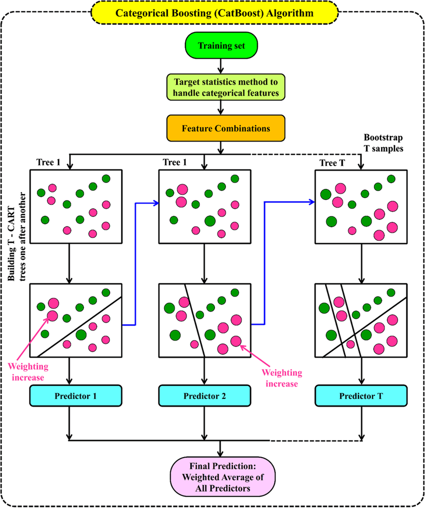
CatBoost
- use Gradient Boosting Decision Tree (GBDT) algorithm
- extra two techniques
- The implementation of ordered boosting, a permutation-driven alternative to the classic algorithm
- An innovative algorithm for processing categorical features
- Main Use Cases
- Good at categorical features, like ecommerce (like product recommendations) and customer behavior analysis
- Inputs
- CSV
- Processes
- xxxxxx
- Hyperparameters
- xxxxxxx
- Instance Types
- only CPUs as memory-bound
LightGBM
- use Gradient Boosting Decision Tree (GBDT) algorithm
- GBDT is a supervised learning algorithm that attempts to accurately predict a target variable by combining an ensemble of estimates from a set of simpler and weaker models
- extra two techniques
- Gradient-based One-Side Sampling (GOSS)
- Exclusive Feature Bundling (EFB)
- Main Use Cases
- ideal for scenarios with large-scale datasets and high-dimensional features, such as in real-time bidding systems, recommendation engines, and large-scale classification problems.
- Inputs
- CSV
- Processes
- xxxxxx
- Hyperparameters
- xxxxxxx
- Instance Types
- only CPUs as memory-bound
| GBDT variants | Strength |
|---|---|
| XGBoost | general use with structured data |
| CatBoost | categorical features |
| LightGBM | large datasets efficiently |
Support Vector Machine (SVM)
- Support Vector Machine (SVM) is a supervised machine learning algorithm that can be employed for both classification and regression purposes. SVM can solve linear and non-linear problems and work well for many practical problems. SVM creates a line or a hyperplane which separates the data into classes.
- SVM is used for text classification tasks such as category assignment, detecting spam and sentiment analysis. It is also commonly used for image recognition challenges, performing particularly well in aspect-based recognition and color-based classification.
- The Support Vector Machines (SVM) is a supervised algorithm mainly used for classification tasks. It uses decision boundaries to separate groups of data.
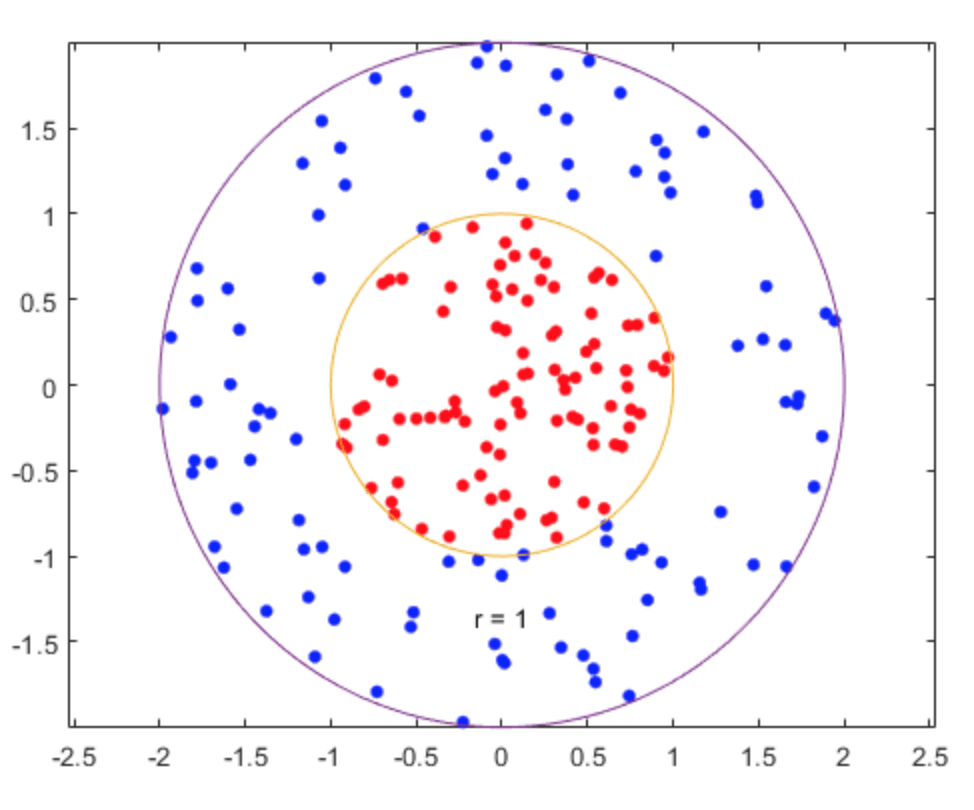
The SVM with Radial Basis Function (RBF) kernel is a variation of the SVM (linear) used to separate non-linear data. Separating randomly distributed data in a two-dimensional space can be a daunting and difficult task. The RBF Kernel provides an efficient way of mapping data (e.g., 2-D) into a higher dimension (e.g, 3-D). In doing so, we can conveniently apply the decision surface/hyperplane where we mainly based our model predictions.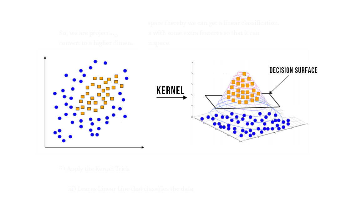
== TEXT ==
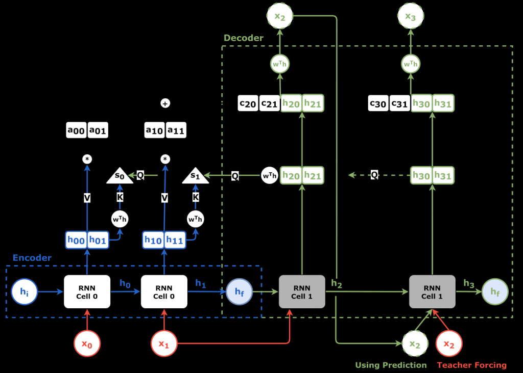
Sequence to Sequence (Seq2Seq) ??
- Input is a sequence of tokens, output is a sequence of tokens
- transform a sequence of elements (such as words in a sentence) into another sequence
- Main Use Cases
- Machine (language) Translation
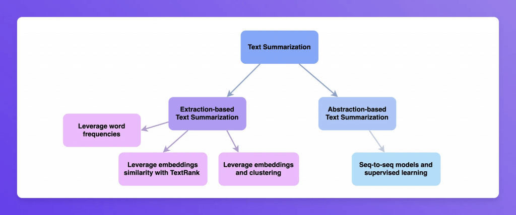
- Text summarization
- Speech to text
- Implemented with RNN’s and CNN’s with attention
- Inputs
- RecordIO-protobuf
- Tokens must be integer, not floating point as others.
- Packs into integer tensors with vocabulary files
- A lot like the TF/IDF lab we did earlier.
- Start with tokenized text files
- Must provide training data, validation data, and vocabulary files.
- RecordIO-protobuf
- Hyperparameters
- Batch_size
- Optimizer_type (adam, sgd, rmsprop)
- Learning_rate
- Num_layers_encoder
- Num_layers_decoder
- Can optimize on:
- Accuracy
- Vs. provided validation dataset
- BLEU score
- Compares against multiple reference translations
- Perplexity
- Cross-entropy
- Accuracy
- Instance Types
- only use GPU instance types
- only use a single machine for training (but can use multiple GPUs)
BlazingText ??
- Main Use Cases
- Predict labels for a sentence <- Word Embedding
- Useful in web searches, information retrieval <- Text Classification
- Modes
- (supervised) Text classification
- Used for perform web searches, information retrieval, ranking, and document classification
- (unsupervised) Word2Vec
- Used for sentiment analysis, named entity recognition, machine translation
- Creates a vector representation of words
- Semantically similar words are represented by vectors close to each other
- This is called a word embedding
- It is useful for NLP, but is not an NLP algorithm in itself!
- Used in machine translation, sentiment analysis
- Remember it only works on individual words, not sentences or documents
- modes
- Cbow (Continuous Bag of Words)
- Skip-gram
- Batch skip-gram
- Distributed computation over many CPU nodes
- (supervised) Text classification
- Input
- For supervised mode (text classification):
- One sentence per line
- First “word” in the sentence is the string “__label__” followed by the label
- Also, “augmented manifest text format”
- Word2vec just wants a text file with one training sentence per line.
- For supervised mode (text classification):
- Hyperparameters
- Text classification:
- Epochs
- Learning_rate
- Word_ngrams
- Vector_dim
- Word2vec:
- Mode (batch_skipgram, skipgram, cbow)
- Learning_rate
- Window_size
- Vector_dim
- Negative_samples
- Text classification:
- Instance Types
- For cbow and skipgram, recommend a single ml.p3.2xlarge
- Any single CPU or single GPU instance will work
- For batch_skipgram, can use single or multiple CPU instances
- For text classification, C5 recommended if less than 2GB training data. For larger data sets, use a single GPU instance (ml.p2.xlarge or ml.p3.2xlarge)
- For cbow and skipgram, recommend a single ml.p3.2xlarge
- Word embedding is a vector representation of a word. Words that are semantically similar correspond to vectors that are close together. That way, word embeddings capture the semantic relationships between words.
Many natural language processing (NLP) applications learn word embeddings by training on large collections of documents. These pre-trained vector representations provide information about semantics and word distributions that typically improve the generalizability of other models that are later trained on a more limited amount of data.
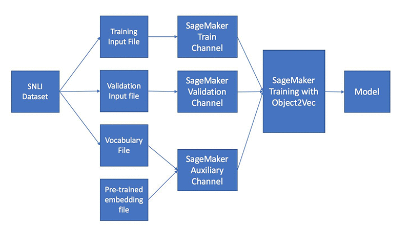
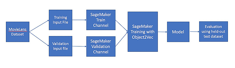
Object2Vec ??
- primarily used for learning vector representations of objects, which can then be used for tasks like similarity search, recommendation, or clustering
- creates low-dimensional dense embeddings of high-dimensional objects
- It is basically word2vec, generalized to handle things other than words.
- for BlazingText Word2Vec, it can find the similiarity among “words”
- for Object2Vec, it can find the similarity among “questions”, “sentences”, “a (long) combinations of words”.
- Compute nearest neighbors of objects
- Main Use Cases
- Visualize clusters
- Genre prediction
- Recommendations (similar items or users)
- Input
- Data must be tokenized into integers
- Training data consists of pairs of tokens and/or sequences of tokens
- Sentence – sentence
- Labels-sequence (genre to description?)
- Customer-customer
- Product-product
- User-item
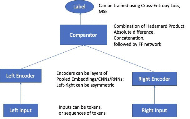
- Processes
- Process data into JSON Lines and shuffle it
- Train with two input channels, two encoders, and a comparator
- Encoder choices:
- Average-pooled embeddings
- CNN’s
- Bidirectional LSTM
- Comparator is followed by a feed-forward neural network
- Hyperparameters
- The usual deep learning ones
- Dropout, early stopping, epochs, learning
rate, batch size, layers, activation
function, optimizer, weight decay
- Dropout, early stopping, epochs, learning
- Enc1_network, enc2_network
- Choose hcnn, bilstm, pooled_embedding
- The usual deep learning ones
- Instance Types
- only train on a single machine (CPU or GPU, multi-GPU OK)
- Inference: use ml.p3.2xlarge
- Use INFERENCE_PREFERRED_MODE environment variable to optimize for encoder embeddings rather than classification or regression.
- the following main components:
Two input channels – The input channels take a pair of objects of the same or different types as inputs, and pass them to independent and customizable encoders.
Two encoders – The two encoders, enc0 and enc1, convert each object into a fixed-length embedding vector. The encoded embeddings of the objects in the pair are then passed into a comparator.
A comparator – The comparator compares the embeddings in different ways and outputs scores that indicate the strength of the relationship between the paired objects. In the output score for a sentence pair. For example, 1 indicates a strong relationship between a sentence pair, and 0 represents a weak relationship.
Pairs of objects are passed through independent, customizable encoders that are compatible with the input types of corresponding objects. The encoders convert each object in a pair into a fixed-length embedding vector of equal length. The pair of vectors are passed to a comparator operator, which assembles the vectors into a single vector using the value specified in the comparator_list hyperparameter. The assembled vector then passes through a multilayer perceptron (MLP) layer, which produces an output that the loss function compares with the labels that you provided. This comparison evaluates the strength of the relationship between the objects in the pair as predicted by the model.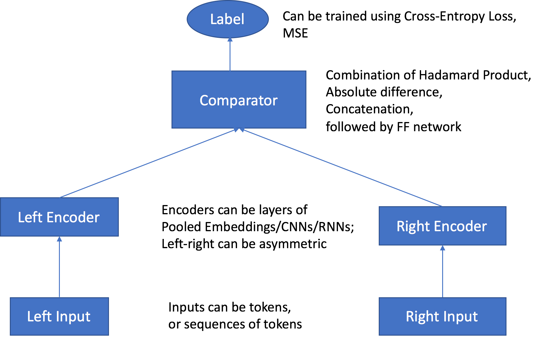
Thedropouthyperparameter refers to the dropout probability for network layers. A dropout is a form of regularization used in neural networks that reduces overfitting by trimming codependent neurons.
This is an optional parameter in Amazon SageMaker Object2vec. Increasing the value of this parameter may say solve the overfitting of the model.

Neural Topic Model (NTM) ???
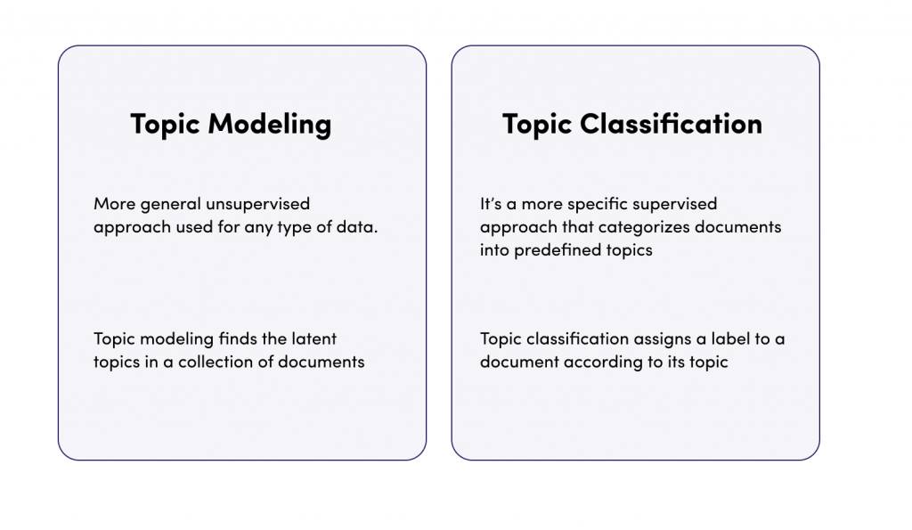
- Organize documents into topics
- Main Use Cases
- Classify or summarize documents based on topics
- Unsupervised
- using “Neural Variational Inference” topic modelling algorithm
- You define how many topics you want
- These topics are a latent representation based on top ranking words
- Input
- Four data channels
- “train” is required
- “validation”, “test”, and “auxiliary” optional
- recordIO-protobuf or CSV
- Words must be tokenized into integers
- Every document must contain a count for every word in the vocabulary in CSV
- The “auxiliary” channel is for the vocabulary
- File or pipe mode
- Four data channels
- Hyperparameters
- Lowering mini_batch_size and learning_rate can reduce validation loss
- At expense of training time
- Num_topics
- Lowering mini_batch_size and learning_rate can reduce validation loss
- Instance Types
- CPU and GPU are all good
- GPU recommended for training
- CPU OK for inference
Latent Dirchlet Allocation (LDA) ????
- Another topic modeling algorithm
- to identify a specified number of topics within a set of text documents
- each document is considered an observation
- the words within the documents are the features
- the topics are the categories
- LDA learns the topics as a probability distribution over the words in the documents, and each document is characterized as a mixture of these topics
- Unsupervised
- The topics themselves are unlabeled; they are just groupings of documents with a shared subset of words
- Main Use Cases
- Can be used for things other than words
- Cluster customers based on purchases
- Harmonic analysis in music
- Can be used for things other than words
- Optional test channel can be used for scoring results
- Per-word log likelihood
- Functionally similar to NTM, but CPU-based
- Therefore maybe cheaper / more efficient
- Input
- Train channel, optional test channel
- recordIO-protobuf or CSV
- Each document has counts for every word in vocabulary (in CSV format)
- Pipe mode only supported with recordIO
- Processing
- Creates a forest of trees where each tree is a partition of the training data; looks at expected change in complexity of the tree as a result of adding a point into it
- Data is sampled randomly
- Then trained
- RCF shows up in Kinesis Analytics as well; it can work on streaming data too.
- Hyperparameters
- Num_topics
- Alpha0
- Initial guess for concentration parameter
- Smaller values generate sparse topic mixtures
- Larger values (>1.0) produce uniform mixtures
- Instance Types
- Single-instance CPU training
== VISION ==
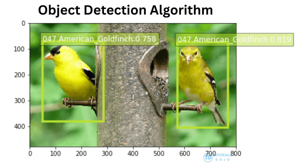
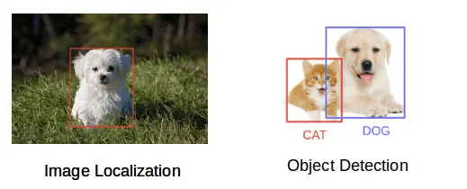
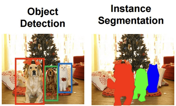
Object Detection
- Takes an image as input, outputs all instances of objects in the image with categories and confidence scores
- Main Use Cases
- Image Object Detection / Identifications
- MXNet
- Uses a CNN with the Single Shot multibox Detector (SSD) algorithm
- The base CNN can be VGG-16 or ResNet-50
- Transfer learning mode / incremental training
- Use a pre-trained model for the base network weights, instead of random initial weights
- Uses flip, rescale, and jitter internally to avoid overfitting
- Uses a CNN with the Single Shot multibox Detector (SSD) algorithm
- Tensorflow
- Uses ResNet, EfficientNet, MobileNet models from the TensorFlow Model Garden
- Input
- MXNet
- RecordIO or image format (jpg or png)
- With image format, supply a JSON file for annotation data for each image
- MXNet
- Hyperparameters
- Mini_batch_size
- Learning_rate
- Optimizer
- Sgd, adam, rmsprop, adadelta
- Instance Types
- Use GPU instances for training (multi-GPU and multi-machine OK)
- Use CPU or GPU for inference
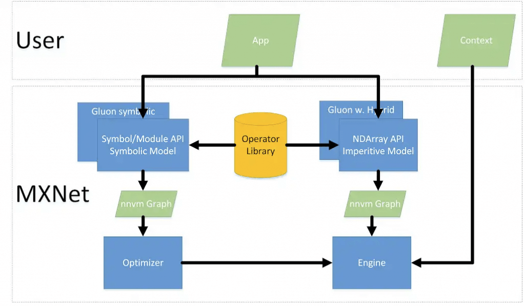
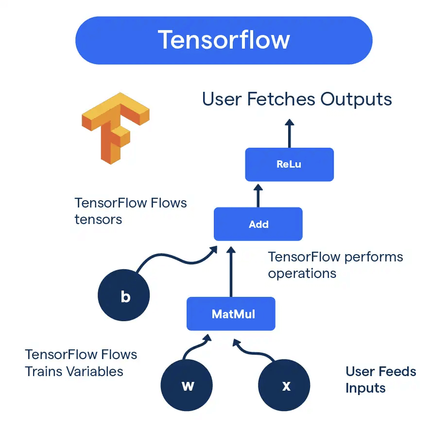
| actor | MXNet | TensorFlow |
| Community Support | Growing community, but smaller compared to TensorFlow | Large and vibrant community with extensive resources |
| Ease of Learning | Slightly steeper learning curve | User-friendly, especially with the Keras API |
| Performance | Efficient and scalable, capable of handling large-scale projects | Slightly slower compared to MXNet for specific tasks |
| Flexibility | Highly flexible in terms of supported languages and hardware | Offers a wide range of tools and supports various hardware options |
| Project Complexity | May require some experience to handle larger projects effectively | Provides best practices and design patterns to manage complexity |
Image Classification
- assigns labels to an entire image, categorizing it based on the predominant features.
- works well for tasks like sorting images into broad categories but cannot identify or count multiple objects within a single image
- a supervised learning algorithm
- Main Use Cases
- Assign one or more labels to an image
- Doesn’t tell you where objects are, just what objects are in the image
- MXNet
- Full training mode
- Network initialized with random weights
- Transfer learning mode
- Initialized with pre-trained weights
- The top fully-connected layer is initialized with random weights
- Network is fine-tuned with new training data
- Default image size is 3-channel 224×224 (ImageNet’s dataset)
- Full training mode
- Tensorflow
- Uses various Tensorflow Hub models (MobileNet, Inception, ResNet, EfficientNet)
- Top classification layer is available for fine tuning or
further training
- Hyperparameters
- The usual suspects for deep learning
- Batch size, learning rate, optimizer
- Optimizer-specific parameters
- Weight decay, beta 1, beta 2, eps, gamma
- Slightly different between MXNet and
Tensorflow versions
- The usual suspects for deep learning
- Instance Types
- Use GPU instances for training (multi-GPU and multi-machine OK)
- Use CPU or GPU for inference
The performance of deep learning neural networks often improves with the amount of data available.
Data augmentation is a technique to artificially create new training data from existing training data. This is done by applying domain-specific techniques to examples from the training data that create new and different training examples.
Image data augmentation is perhaps the most well-known type of data augmentation and involves creating transformed versions of images in the training dataset that belong to the same class as the original image.

Training deep learning neural network models on more data can result in more skillful models, and the augmentation techniques can create variations of the images that can improve the ability of the fit models to generalize what they have learned to new images.
Semantic Segmentation
- Pixel-level object classification
- classifies each pixel in an image into different categories, providing a detailed map of where different objects or materials are located within the image
- Different from image classification – that assigns labels to whole images
- Different from object detection – that assigns labels to bounding boxes
- Main Use Cases
- self-driving vehicles
- medical imaging diagnostics
- robot sensing
- Produces a segmentation mask
- Built on MXNet Gluon and Gluon CV
- Choice of 3 algorithms:
- Fully-Convolutional Network (FCN)
- Pyramid Scene Parsing (PSP)
- DeepLabV3
- Choice of backbones:
- ResNet50
- ResNet101
- Both trained on ImageNet
- Incremental training, or training from scratch, supported too
- Input
- JPG Images and PNG annotations
- For both training and validation
- Label maps to describe annotations
- Augmented manifest image format supported for Pipe mode.
- JPG images accepted for inference
- Hyperparameters
- Epochs, learning rate, batch size, optimizer, etc
- Algorithm
- Backbone
- Instance Types
- Use GPU instances for training (multi-GPU and multi-machine OK)
- Use CPU or GPU for inference
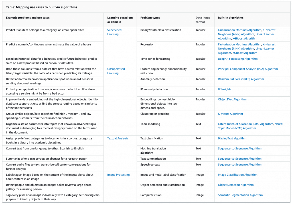
| Data type | supervised | unsupervised | |
|---|---|---|---|
| Binary/Multiple – Classification (Predict if an item belongs to a category: an email spam filter) | Tabular | – Linear Learner Algorithm – K-Nearest Neighbors (k-NN) – Factorization Machines – AutoGluon-Tabular – TabTransformer – XGBoost – CatBoost – LightGBM | |
| Regression (Predict a numeric/continuous value: estimate the value of a house) | Tabular | – Linear Learner Algorithm – K-Nearest Neighbors (k-NN) – Factorization Machines – AutoGluon-Tabular – TabTransformer – XGBoost – CatBoost – LightGBM | |
| Time-series forecasting (Based on historical data for a behavior, predict future behavior: predict sales on a new product based on previous sales data.) | Tabular | DeepAR | |
| Feature engineering: dimensionality reduction (Drop those columns from a dataset that have a weak relation with the label/target variable: the color of a car when predicting its mileage.) | Tabular | Principal Component Analysis (PCA) | |
| Anomaly detection (Detect abnormal behavior in application: spot when an IoT sensor is sending abnormal readings) | Tabular | Random Cut Forest (RCF) | |
| Clustering or grouping (Group similar objects/data together: find high-, medium-, and low-spending customers from their transaction histories) | Tabular | K-Means | |
| IP Address Pattern / IP anomaly detection (Protect your application from suspicious users: detect if an IP address accessing a service might be from a bad actor) | Tabular | IP Insights | |
| Language Translation (Convert text from one language to other: Spanish to English) | Text | Seq2Seq | |
| Text summarization (Summarize a long text corpus: an abstract for a research paper) | Text | Seq2Seq | |
| Speech-to-text (Convert audio files to text: transcribe call center conversations for further analysis) | Text | Seq2Seq | |
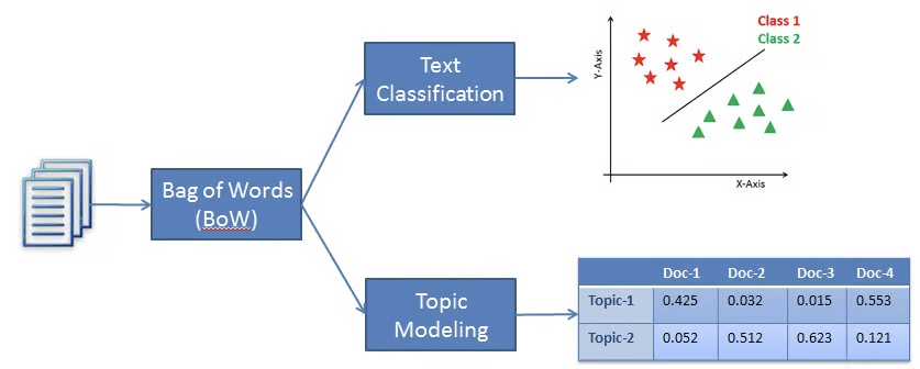
| Text Classification (Assign pre-defined categories to documents in a corpus: categorize books in a library into academic disciplines) | Text | BlazingText, Text Classification – TensorFlow | |
| Topic Modeling/Discovery (Organize a set of documents into topics (not known in advance): tag a document as belonging to a medical category based on the terms used in the document.) | Text | Latent Dirichlet Allocation (LDA), Neural Topic Model (NTM) | |
| Dense Embeddings / Feature Engineering (Improve the data embeddings of the high-dimensional objects: identify duplicate support tickets or find the correct routing based on similarity of text in the tickets) | Text | Object2Vec | |
| Image and multi-label classification (Label/tag an image based on the content of the image: alerts about adult content in an image) | Image | Image Classification – MXNet | |
| Image classification (Classify something in an image using transfer learning.) | Image | Image Classification – TensorFlow | |
| Computer vision (Tag every pixel of an image individually with a category: self-driving cars prepare to identify objects in their way) | Image | Semantic Segmentation | |
| Object detection and classification (Detect people and objects in an image: police review a large photo gallery for a missing person) | Image | Object Detection – MXNet, Object Detection – TensorFlow |
== REINFORCEMENT ==
Reinforcement Learning
- You have some sort of agent that “explores” some space
- As it goes, it learns the value of different state changes in different conditions
- Those values inform subsequent behavior of the agent
- Examples: Pac-Man, Cat & Mouse game (game AI)
- Supply chain management
- HVAC systems
- Industrial robotics
- Dialog systems
- Autonomous vehicles
- Yields fast on-line performance once the space has been explored
- Q-Learning
- A set of environmental states s
- A set of possible actions in those states a
- A value of each state/action Q
- Start off with Q values of 0
- Explore the space
- As bad things happen after a given state/action, reduce its Q
- As rewards happen after a given state/action, increase its Q
- can “look ahead” more than one step by using a discount factor when computing Q (here s is previous state, s’ is current state)
- Q(s,a) += discount * (reward(s,a) + max(Q(s’)) – Q(s,a))
- The exploration problem
- efficiently explore all of the possible states
- Simple approach: always choose the action for a given state with the highest Q. If there’s a tie, choose at random
- But that’s really inefficient, and you might miss a lot of paths that way
- Better way: introduce an epsilon term
- If a random number is less than epsilon, don’t follow the highest Q, but choose at random
- That way, exploration never totally stops
- Choosing epsilon can be tricky
- Markov Decision Process (MDP)
- modeling decision making in situations where outcomes are partly random and partly under the control of a decision maker
- States are still described as s and s’
- State transition functions are described as 𝑃𝑎 (𝑠, 𝑠′)
- Our “Q” values are described as a reward function 𝑅𝑎 (𝑠, 𝑠′)
- a discrete time stochastic control process.
- modeling decision making in situations where outcomes are partly random and partly under the control of a decision maker
- RL in SageMaker
- Uses a deep learning framework with Tensorflow and MXNet
- Supports Intel Coach and Ray Rllib toolkits.
- MATLAB, Simulink
- EnergyPlus, RoboSchool, PyBullet
- Amazon Sumerian, AWS RoboMaker
- Distributed Training with SageMaker RL
- Can distribute training and/or environment rollout
- Multi-core and multi-instance
- Key Terms
- Environment
- The layout of the board / maze / etc
- State
- Where the player / pieces are
- Action
- Move in a given direction, etc
- Reward
- Value associated with the action from that state
- Observation
- i.e., surroundings in a maze, state of chess board
- Environment
- Hyperparameters
- Parameters of your choosing may be abstracted
- Hyperparameter tuning in SageMaker can then optimize them
- Instance Types
- deep learning – so GPU’s are helpful
- supports multiple instances and cores
Multinomial logistic regression is used to predict categorical placement in or the probability of category membership on a dependent variable based on multiple independent variables.
It is a simple extension of binary logistic regression that allows for more than two categories of the dependent or outcome variable. Like binary logistic regression, multinomial logistic regression uses maximum likelihood estimation to evaluate the probability of categorical membership.
A baseline model is a model that is easy and simple to set up and one that can deliver fair results. In this scenario, Multinomial Logistic Regression would be the best option as it’s reasonably simple and effective.
Latent Dirichlet Allocation (LDA) is incorrect because this algorithm is primarily used for topic modeling.
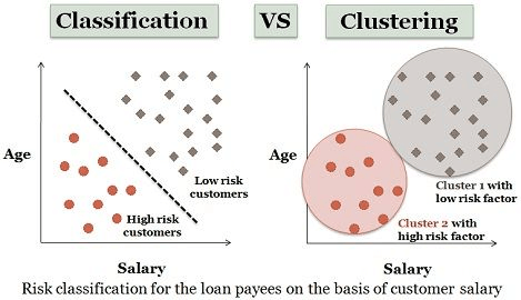
K-means Clustering is incorrect. This is an unsupervised algorithm that attempts to find discrete groupings within data, where members of a group are as similar as possible to one another and as different as possible from members of other groups. This algorithm won’t work because we’re dealing with a labeled dataset. What we need here is a supervised classification algorithm since we’re just classifying data into known categories.
Recurrent Neural Network (RNN) is incorrect. This will likely perform better than Multinomial Logistic Regression, but it won’t fit the requirement as we only need to come up with a baseline model. RNN would be too complex to set up.
Multiclass classification is related to two other machine learning tasks, binary classification and the multilabel problem. Binary classification is already supported by linear learner, and multiclass classification is now available with linear learner, but multilabel support is not yet available from linear learner.
If there are only two possible labels in your dataset, then you have a binary classification problem. Examples include predicting whether a transaction will be fraudulent or not based on transaction and customer data, or detecting whether a person is smiling or not based on features extracted from a photo. For each example in your dataset, one of the possible labels is correct and the other is incorrect. The person is smiling or not smiling.
If there are more than two possible labels in your dataset, then you have a multiclass classification problem. For example, predicting whether a transaction will be fraudulent, cancelled, returned, or completed as usual. Or detecting whether a person in a photo is smiling, frowning, surprised, or frightened. There are multiple possible labels, but only one is correct at a time.
If there are multiple labels, and a single training example can have more than one correct label, then you have a multilabel problem. For example, tagging an image with tags from a known set. An image of a dog catching a Frisbee at the park might be labeled as outdoors, dog, and park. For any given image, those three labels could all be true, or all be false, or any combination. Although we haven’t added support for multilabel problems yet, there are a couple of ways you can solve a multilabel problem with linear learner today. You can train a separate binary classifier for each label. Or you can train a multiclass classifier and predict not only the top class, but the top k classes, or all classes with probability scores above some threshold.
Linear learner uses a softmax loss function to train multiclass classifiers. The algorithm learns a set of weights for each class, and predicts a probability for each class. We might want to use these probabilities directly, for example if we’re classifying emails as inbox, work, shopping, spam and we have a policy to flag as spam only if the class probability is over 99.99%. But in many multiclass classification use cases, we’ll simply take the class with highest probability as the predicted label.