19. ML – Data Science Extend

=== MODEL PRACTICE ===

Text (Classification) Models

• Low Accuracy, due to a rich vocabulary plus a low average frequency of words
  • Term Frequency – Inverse Document Frequency (TfIdf) is an algorithm used to convert text data into its numerical representation that can be passed into a machine learning model. The first function (Term Frequency) counts how frequently a word appears in a sentence belonging to a corpus. The second function (Inverse Document Frequency) counts how frequently a word appears in the whole corpus.
    The Tf-Idf is a great way of giving weights to words as it penalizes generic words that commonly appear across all sentences.
    Consider the example below: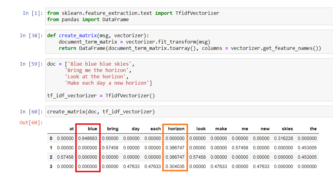
    
    In the example, we have 4 sentences inside a document. The word “blue” is only present in the first sentence, while the word “horizon” is present in 3 sentences. Notice how the word “blue” and “horizon” each appears 3 times in the whole document, but the “blue” has more weight compared to the “horizon”. Even if a word has a low frequency across all documents, the Tf-Idf vectorizer is still able to capture how special that word is by giving it a higher score.
  • Solution: Use the Scikit-learn TfidfVectorizer Class
  • Relevant but not appropriate
    • Stemming and Stop word removal has nothing to do with how frequently a word appears in a document. Stemming is just a process of reducing a word into its root/stem word (e.g., tokenization -> token) while Stop word removal is a process of removing words that don’t convey too much important meaning in a sentence (e.g., is, at, are.)
• Text cleaning/text preprocessing is an integral stage of an NLP pipeline
  • you have to give “structure” to them so they can be conveniently processed and understood by your model.
    
  • Some examples of preprocessing are Changing letters into lowercase, Word Tokenization, Stop word removal, HTML tag removal, Stemming, Lemmatization, and so on.
    • Changing letters into lowercase will bring uniformity to all available data.
    • Stop word removal is the process of removing words that do not hold any significant meaning to a sentence. These are words that are commonly used and repeated (e.g., the, is, are). Removing them will reduce the overall size of your data which will eventually help speed up model training.
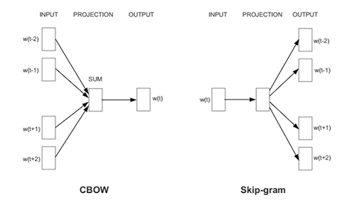
    • Word Tokenization is the process of splitting a sentence into individual words that can be used as input for the Word2vec model to create embeddings.

Classification Models

• Binary classification model with requirements
  • Choose the most cost-effective model given that false negatives are 3 times more expensive than false positives.
  • Choose the model with a recall rate of 85% or more.
  • Choose the model with a false negative rate of 15% or less.
  • To correctly answer this problem, we have to know three formulas:
    -> Recall = TP / (TP+FN)
-> False Negative Rate = FN / (FN+TP)
    The cost function is dictated by our business problem. Note that every problem has different needs and therefore will require different cost functions.
    It is stated in the scenario that false negatives are 3 times costlier than false positives.
    If we translate that into an equation, we’ll arrive at:
    -> Cost Function = (3 * FN) + FP
    The full table summary of the calculated values is shown below: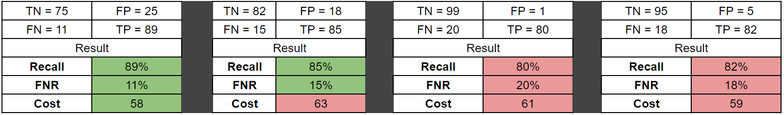
    
• Another Binary
  • The model was evaluated on a test dataset of 100 customers. The confusion matrix for the model is given below:
    
    
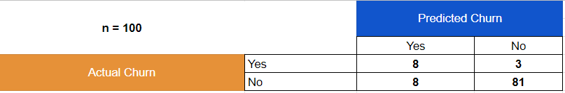
    Accuracy measures the fraction of correct predictions. The range is 0 to 1. A larger value indicates better predictive accuracy. It is computed by dividing the sum of True Positives and True Negatives by the total number of predictions.
  • To solve for Accuracy, let us first identify the four statistics of the model’s confusion matrix:
  • TP = 8, TN = 81, FP = 8, FN = 3
  • Accuracy = (TP + TN ) / (TP + TN + FP + FN)
  • Accuracy = (8 + 81)/(100) = 0.89 x 100 = 89%
  • Hence, the accuracy of this model is 89%.
  • For this type of business problem, minimizing the False Negatives should be the top priority because they incorrectly predict that a churning customer will stay. In simple terms, this is the costliest among the four as you’d lose $50 for every erroneous prediction.
  • The False Positives represent happy customers that the model mistakenly predicted to churn. This means that you’re wasting a retention incentive of $3 for customers who don’t have the tendency to cancel subscriptions.
  • Let’s calculate the loss to the company without the retention incentive:
  • Loss due to actual churn = (8 + 3) * $50 = $550
  • Now, let’s see what would happen if the model is deployed and the retention incentive is in effect:
  • Total loss = $50 * FN + $0 * TN + $3 * FP(C) + $3 * TP = $50(3) + $0(81) + $3(8) + $3(8) = $198
  • Because the total loss is less when the model is deployed than when it is not, the model is feasible to deploy in production.
  • Hence, the correct answer is: Yes. The model’s accuracy is 89%. The total loss is less when the model is deployed than when it is not.
• Three Categories Modal
  • The confusion matrix
    
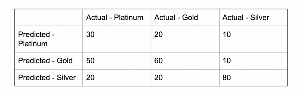
    The actual output of a multi-class classification algorithm is a set of prediction scores. The scores indicate the model’s certainty that the given observation belongs to each of the classes. Unlike for binary classification problems, you do not need to choose a score cut-off to make predictions. The predicted answer is the class (for example, label) with the highest predicted score.
    Need to calculate for each category, and get the average
    Accuracy: (TP + TN) / (P + N) Accuracy for Platinum = ((30+(60+80))/(30+20+10+50+60+10+20+20+80)) = 170/200 = 0.85
    Accuracy for Gold = ((60+(30+80))/(30+20+10+50+60+10+20+20+80)) = 170/200 = 0.85
    Accuracy for Silver = ((80+(60+30))/(30+20+10+50+60+10+20+20+80)) = 170/200 = 0.85
    Overall Accuracy = Average of the accuracy for Platinum, Gold and Silver = (0.85+0.85+0.85)/3 = 0.85
    Precision: TP / (TP + FP) Precision for Platinum = (30/(30+ (20+10))) = 30/60 = 0.50
    Precision for Gold = (60/(60+ (50+10))) = 60/120 = 0.50
    Precision for Silver = (80/(80+ (20+20))) = 80/120 = 0.67
    Overall Precision = Average of the precision for Platinum, Gold and Silver = (0.50+0.50+0.67)/3 = 0.56
    Recall / Sensivity: TP / (TP + FN) Recall for Platinum = (30/(30+(50+20))) = 30/100 = 0.30
    Recall for Gold = (60/(60+(20+20))) = 60/100 = 0.60
    Recall for Silver = (80/(80+10+10)) = 80/100 = 0.80
    Overall Recall = Average of the recall for Platinum, Gold and Silver = (0.30+0.60+0.80)/3 = 0.57
    F1-Score: 2TP / (2TP + FP + FN) F1-Score for Platinum = (2*30/(2*30+(20+10)+(50+20))) = 60/160 = 0.38
    F1-Score for Gold = (2*60/(2*60+(50+10)+(20+20))) = 120/220 = 0.55
    F1-Score for Silver = (2*80/(2*80+(60+30)+(10+10))) = 160/270 = 0.59
    Overall F1-Score = Average of the F1-Score for Platinum, Gold and Silver = (0.38+0.55+0.59)/3 = 0.51
• KNN
  • Most k-NN models use the Euclidean distance to measure how similar the target data is to a specific class. Since the Euclidean distance is a function of data points in a graph, the position of our data points greatly influences the resulting Euclidean distance. Consider a dataset with a feature called ‘age’ that ranges between 18-35 and a ‘product price’ that ranges between $50 – $5,000. Since the product price has a significantly larger value than the age, the model will treat the product price with “more importance”. This would have a negative impact on the model’s ability to classify data correctly.

Numeric Models

• Time Series Forecast
  • One key concept in these predictions is the use of quantiles, which are specific probabilities associated with forecasted values.
  • A quantile in forecasting represents the value below which a certain percentage of the data points will fall. In the context of time-series forecasting in Amazon SageMaker Clarify, quantiles help address the uncertainty in predictions by giving a range of potential outcomes rather than a single point estimate. For example:
    – P10 represents the forecast value where 10% of the possible outcomes will fall below it, meaning it’s a conservative prediction of lower demand.
    – P50 represents the median forecast, where 50% of the possible outcomes will fall below it. This is a balanced estimate, assuming equal likelihood of underestimating or overestimating demand.
    – P90 or P99 represent higher quantiles, where 90% or 99% of the outcomes fall below the forecasted value, offering a more conservative and high-end estimate for situations where understocking or under-preparation would be costly.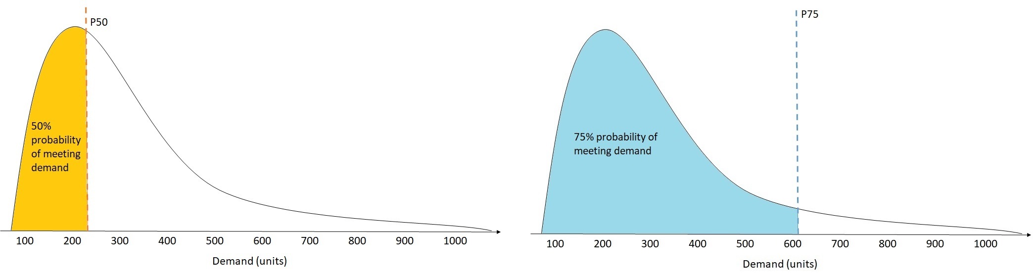
    

Image Models

• To achieve higher accuracy, it’s also common to use data augmentation in addition to transfer learning. It’s the fastest and cheapest way to multiply the amount of training data you have by generating new data based on your existing training data.
• For example, you can perform augmentation by flipping the image or rotating them 90 degrees clockwise and counterclockwise

Model Tuning

• The specified range of values for the learning rate is between .0001 and 1.0.
  • By default, SageMaker assumes a uniform distribution of hyperparameter values and uses linear scaling to select values in a search range. However, this may not be the most effective approach for some types of hyperparameters, such as a learning rate whose typical value spans multiple orders of magnitude and is not uniformly distributed. Customers can either rely on SageMaker to automatically determine the scaling method or manually select it, for each hyperparameter to be tuned.
    During hyperparameter tuning, SageMaker attempts to figure out if your hyperparameters are log-scaled or linear-scaled. Initially, it assumes that hyperparameters are linear-scaled. If they are in fact log-scaled, it might take some time for SageMaker to discover that. If you know that a hyperparameter is log-scaled and can convert it yourself, doing so could improve hyperparameter optimization.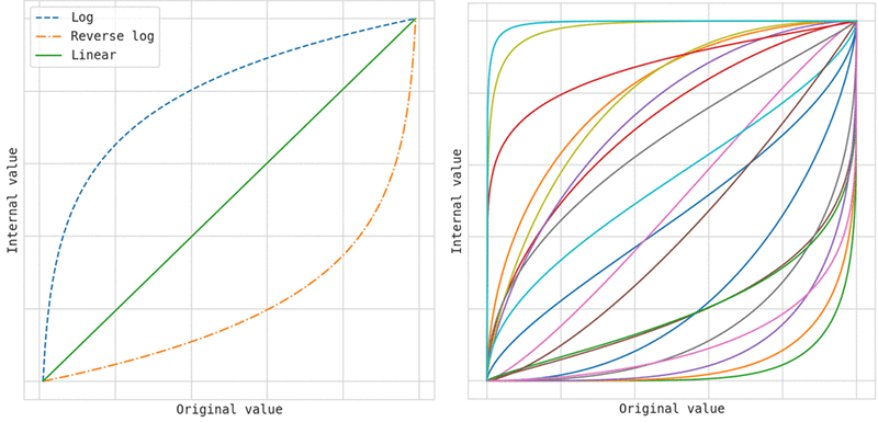
    
    Logarithmic scaling works only for ranges that have only values greater than 0. Choose logarithmic scaling when you are searching for a range that spans several orders of magnitude. For example, if you are tuning a linear learner model and you specify a range of values between .0001 and 1.0 for the learning_rate hyperparameter, searching uniformly on a logarithmic scale gives you a better sample of the entire range than searching on a linear scale would. This is because searching on a linear scale would, on average, devote 90 percent of your training budget to only the values between .1 and 1.0, leaving only 10 percent of your training budget for the values between .0001 and .1.
• the loss function is oscillating
  • The learning rate is a constant value used in the Stochastic Gradient Descent (SGD) algorithm. Learning rate affects the speed at which the algorithm reaches (converges to) the optimal weights. The SGD algorithm makes updates to the weights of the linear model for every data example it sees. The size of these updates is controlled by the learning rate.
    
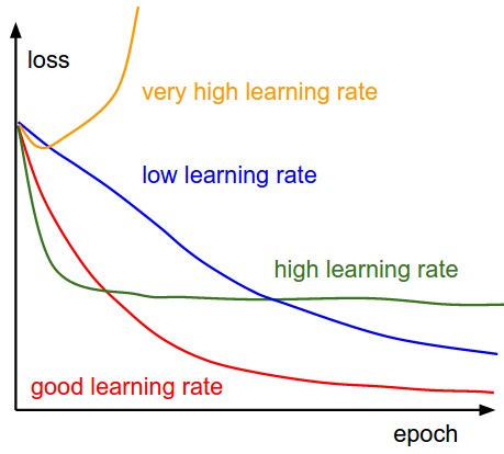
    Too large a learning rate might prevent the weights from approaching the optimal solution. Too small a value results in the algorithm requiring many passes to approach the optimal weights. In Amazon ML, the learning rate is auto-selected based on your data.
    A Loss function evaluates how effective an algorithm is at modeling the data. For example, if a model consistently predicts values that are very different from the actual values, it returns a large loss. Depending on the training algorithm, more than one loss function might be used.
• Early Stop
  • Stopping training jobs early can help reduce compute time and helps you avoid overfitting your model.
    
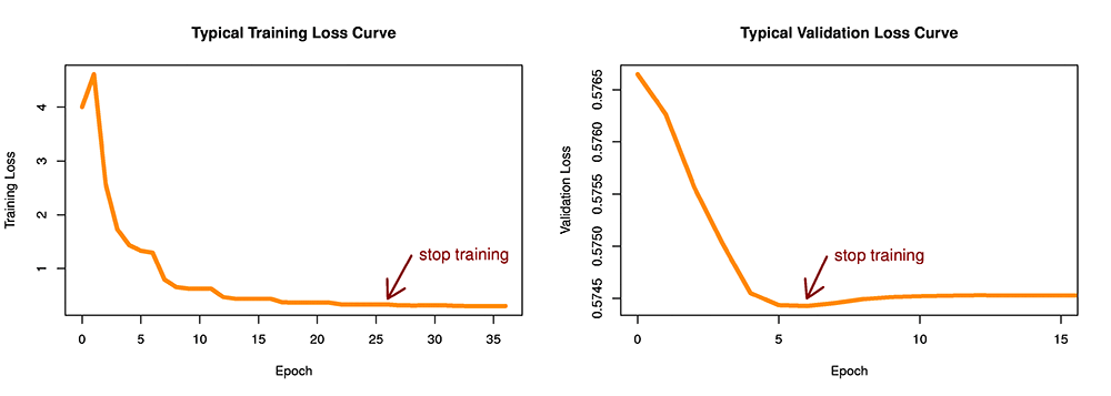
    When you enable early stopping for a hyperparameter tuning job, SageMaker evaluates each training job that the hyperparameter tuning job launches as follows:
    – After each epoch of training, get the value of the objective metric.
    – Compute the running average of the objective metric for all previous training jobs up to the same epoch, and then compute the median of all of the running averages.
    – If the value of the objective metric for the current training job is worse (higher when minimizing or lower when maximizing the objective metric) than the median value of running averages of the objective metric for previous training jobs up to the same epoch, SageMaker stops the current training job.
    To use early stopping with your own algorithm, you must write your algorithms such that it emits the value of the objective metric after each epoch.
• Tune the model performance
  • You can fine-tune your ML model performance metrics by adjusting the score threshold. Adjusting this value changes the level of confidence that the model must have in a prediction before it considers the prediction to be positive. It also changes how many false negatives and false positives you are willing to tolerate in your predictions.
    
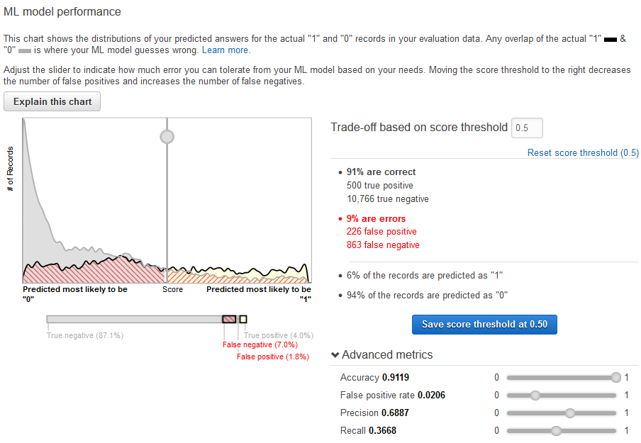
    You can control the cutoff for what the model considers a positive prediction by increasing the score threshold until it considers only the predictions with the highest likelihood of being true positives as positive. You can also reduce the score threshold until you no longer have any false negatives. Choose your cutoff to reflect your business needs.
• Model Pruning
  • Model pruning aims to remove weights that don’t contribute much to the training process. Weights are learnable parameters: they are randomly initialized and optimized during the training process. During the forward pass, data passes through the model. The loss function evaluates model output given the labels; during the backward pass, weights are updated to minimize the loss. To do so, the gradients of the loss with respect to the weights are computed, and each weight receives a different update.
    
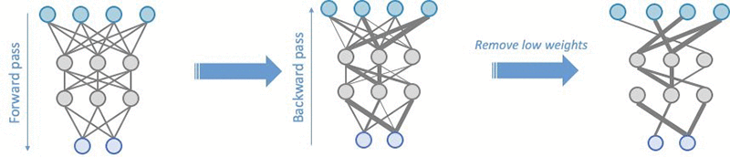
    After a few iterations, certain weights are typically more impactful than others; the g

——

In transfer learning, the network is initialized with pre-trained weights and just the top fully connected layer is initialized with random weights. Then, the whole network is fine-tuned with new data. In this mode, training can be achieved even with a smaller dataset. This is because the network is already trained and therefore can be used in cases without sufficient training data.

In the scenario, the model begins with some basic understanding of the Japanese language. This helps the model recognize patterns in the language. Now, we want this model to specifically identify if a sentence is grammatically right or wrong. To do this, we train a special classifier and then replace the part of the model that makes the final decision with this new classifier. This way, we’re fine-tuning the model to be good at recognizing whether Japanese sentences follow the grammar rules or not.

——

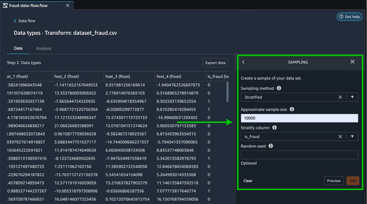
Stratified sampling is a method used to divide a dataset into subsets (strata) where each subset represents the class proportions of the original dataset. This ensures that both the training and validation datasets maintain the same class distribution as the overall dataset. It is particularly useful when dealing with imbalanced datasets, where certain classes are overrepresented or underrepresented compared to others.

——

Amazon API Gateway is a fully managed service that makes it easy for developers to create, publish, maintain, monitor, and secure APIs at any scale. API Gateway can be used to present an external-facing, single point of entry for Amazon SageMaker endpoints.

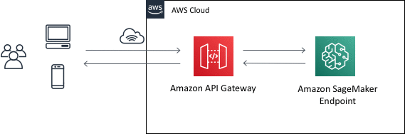
API Gateway can be used to front an Amazon SageMaker inference endpoint as (part of) a REST API, by making use of an API Gateway feature called mapping templates. With mapping templates, you can use Velocity Template Language (VTL) templates to convert from the REST request format to the model input format, and to convert the model output to the REST response format. 

——

Amazon SageMaker Debugger comes with built-in analytics that automatically analyzes data emitted during training, such as inputs, outputs, and transformations known as tensors.

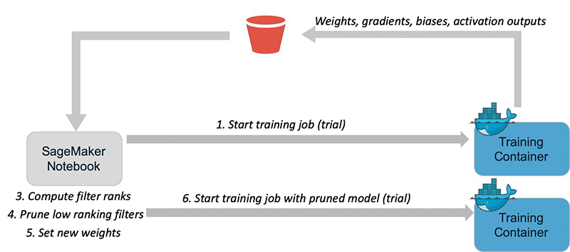
Once you retrieve the emitted tensors, you can determine the importance of each filter by accumulating the product of activation outputs and gradients throughout the training. You then remove the lowest-ranked filters and fine-tune the model to recover from the pruning and regain accuracy. You can repeat these steps several times to optimize the model.

By pruning the model, the company can reduce the model’s size while maintaining its accuracy, allowing for faster prediction times.

Hence, the correct answer is: In the training script, include a SageMaker Debugger hook that collects information on a tensor of weights, gradients, biases, and activation outputs. Compute filter ranks based on these tensors to identify low-ranking filters. Prune low-ranking filters and make weight adjustments. Retrain the pruned model.

The option that says: Train the dataset using Amazon SageMaker Autopilot to automatically search for the model with the highest accuracy is incorrect. The scenario specifically mentions using a pre-trained CNN model and fine-tuning it for the task of car damage assessment. SageMaker Autopilot is designed to search for the best model based on a given dataset, but it does not directly support using pre-trained models and fine-tuning them. Additionally, SageMaker Autopilot only supports tabular data such as CSV and Parquet, not images.

—–

Your model is underfitting the training data when the model performs poorly on the training data. This is because the model is unable to capture the relationship between the input examples (often called X) and the target values (often called Y).

Poor performance on the training data could be because the model is too simple (the input features are not expressive enough) to describe the target well. Performance can be improved by increasing model flexibility. To increase model flexibility, try the following:

• Add new domain-specific features and more feature Cartesian products, and change the types of feature processing used (e.g., increasing n-grams size)
• Decrease the amount of regularization used.

If your model is overfitting the training data, it makes sense to take actions that reduce model flexibility. To reduce model flexibility, try the following:

• Feature selection: consider using fewer feature combinations, decrease n-grams size, and decrease the number of numeric attribute bins.
• Increase the amount of regularization used.

Accuracy on training and test data could be poor because the learning algorithm did not have enough data to learn from. You could improve performance by doing the following:

• Increase the amount of training data examples.
• Increase the number of passes on the existing training data.

—-

Regularization helps prevent linear models from overfitting training data examples (that is, memorizing patterns instead of generalizing them) by penalizing extreme weight values. L1 regularization has the effect of reducing the number of features used in the model by pushing to zero the weights of features that would otherwise have small weights.

As a result, L1 regularization results in sparse models and reduces the amount of noise in the model. L2 regularization results in smaller overall weight values and stabilizes the weights when there is a high correlation between the input features. You control the amount of L1 or L2 regularization applied by using the Regularization type and Regularization amount parameters. An extremely large regularization value could result in all features having zero weights, preventing a model from learning patterns.

In the scenario, the model is overfitting since an increase in epoch number causes a sharp decrease in the training error rate. In this case, it makes sense to use regularization techniques to prevent the model from overfitting.

——

Deep neural networks contain multiple non-linear hidden layers and this makes them very expressive models that can learn very complicated relationships between their inputs and outputs. With limited training data, however, many of these complicated relationships will be the result of sampling noise, so they will exist in the training set but not in real test data even if it is drawn from the same distribution. This leads to overfitting and many methods have been developed for reducing it.

Dropout is a technique that addresses this issue. It prevents overfitting and provides a way of approximately combining exponentially many different neural network architectures efficiently. The term dropout refers to dropping out units (hidden and visible) in a neural network.

——

The Bayesian optimization is a sequential algorithm that learns from past trainings as the tuning job progresses. This tuning algorithm learns from each incremental step which highly limits parallelism.

Running more hyperparameter tuning jobs concurrently gets more work done quickly, but a tuning job improves only through successive rounds of experiments. Typically, running one training job at a time achieves the best results with the least amount of compute time.

---

=== XXXXXXX ===

Pose estimation

• a computer vision technique that identifies a collection of points on objects, such as people or vehicles, in images or videos. This method has various real-world applications, including in sports, robotics, security, augmented reality, media and entertainment, and medical fields. Pose estimation models are trained using images or videos that have been annotated with a consistent set of points (coordinates) defined by a specific rig. This is critical for analyzing how vehicles and pedestrians move and interact in the busy intersection. Amazon SageMaker AI supports training and deployment of Pose Estimation models with managed infrastructure, ensuring minimal operational overhead while achieving high accuracy for motion analysis.
  

——

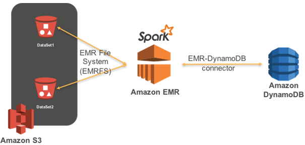
Amazon EMR is the best place to run Apache Spark. You can quickly and easily create managed Spark clusters from the AWS Management Console, AWS CLI, or the Amazon EMR API. Apache Spark includes several libraries to help build applications for machine learning (MLlib), stream processing (Spark Streaming), and graph processing (GraphX).

Collaborative filtering is based on (user, item, rating) tuples. So, unlike content-based filtering, it leverages other users’ experiences. The main concept behind collaborative filtering is that users with similar tastes (based on observed user-item interactions) are more likely to have similar interactions with items they haven’t seen before.

Compared to content-based filtering, collaborative filtering provides better results for diversity (how dissimilar recommended items are); serendipity (a measure of how surprising the successful or relevant recommendations are); and novelty (how unknown recommended items are to a user).

The content-based filtering algorithm is more suited for making predictions based on the product’s attributes.

—–

Amazon Redshift ML makes it easy for data analysts and database developers to create, train, and apply machine learning models using familiar SQL commands in Amazon Redshift data warehouses. With Redshift ML, you can take advantage of Amazon SageMaker without learning new tools or languages. Simply use SQL statements to create and train Amazon SageMaker machine learning models using your Redshift data and then use these models to make predictions.

For example, you can use customer retention data in Redshift to train a churn detection model and then apply that model to your dashboards for your marketing team to offer incentives to customers at risk of churning. Redshift ML makes the model available as a SQL function within your Redshift data warehouse so you can easily apply it directly in your queries and reports.

In the scenario, by using Redshift ML, the input data can be processed directly within the Redshift cluster, reducing the time and resources required to move data between Redshift and Amazon S3. Additionally, Redshift ML is designed to perform fast, in-database machine learning, which can help speed up the prediction generation process and reduce the overall cost of inference.

Online Reference: