Deep Learning
- Frameworks
- Tensorflow / Keras
- MXNet
- Types of Neural Networks
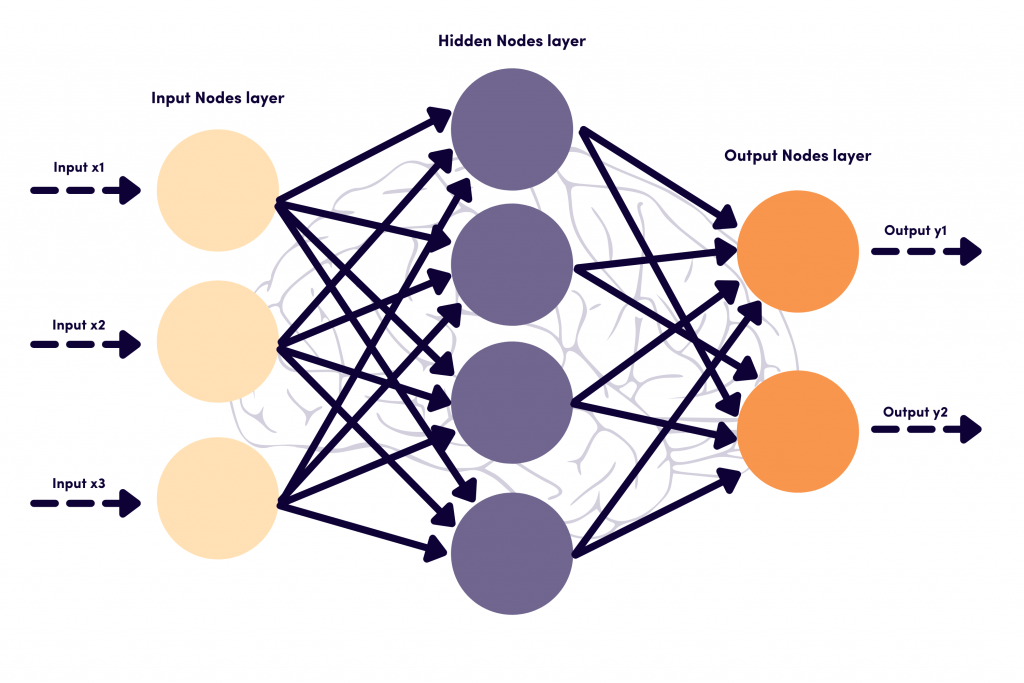
- Feedforward Neural Network (FFNN)
- from one layer to another without touching a node twice
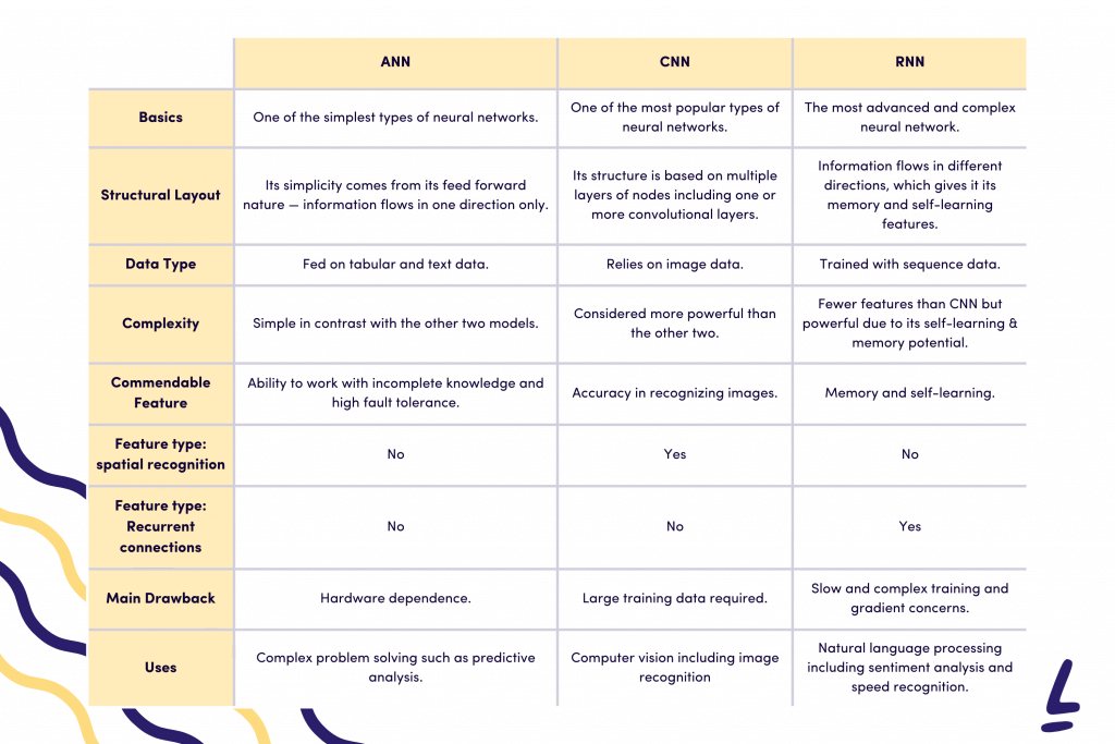
- Artificial Neural Networks (ANN)
- Convolutional Neural Networks (CNN)
- used for Computer Vision (image and video recognition, recommendation systems, and image analysis and classification)
- Image classification (is there a stop sign in this image?)
- using linear algebra principles to identify patterns in images.
- Convolutional layer
- Pooling layer
- Fully-connected layer
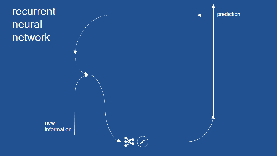
- Recurrent Neural Networks (RNNs)
- Deals with sequences in time (predict stock prices, understand words in a sentence, translation, etc); mostly with Natural Language Processing.
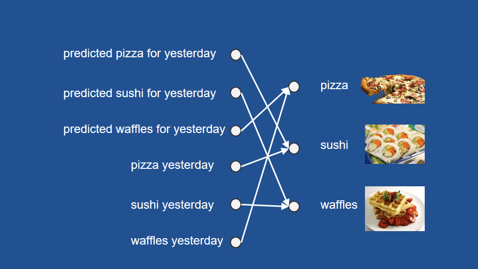
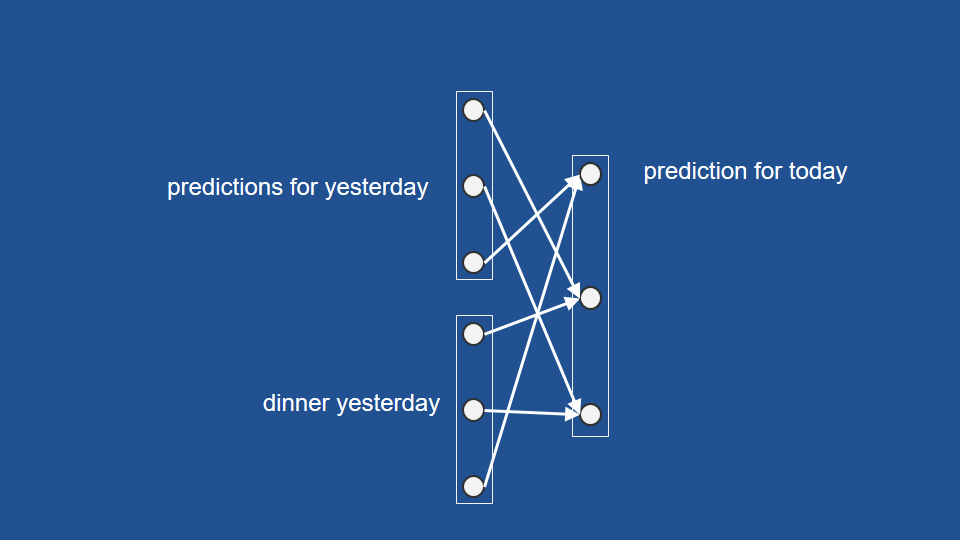
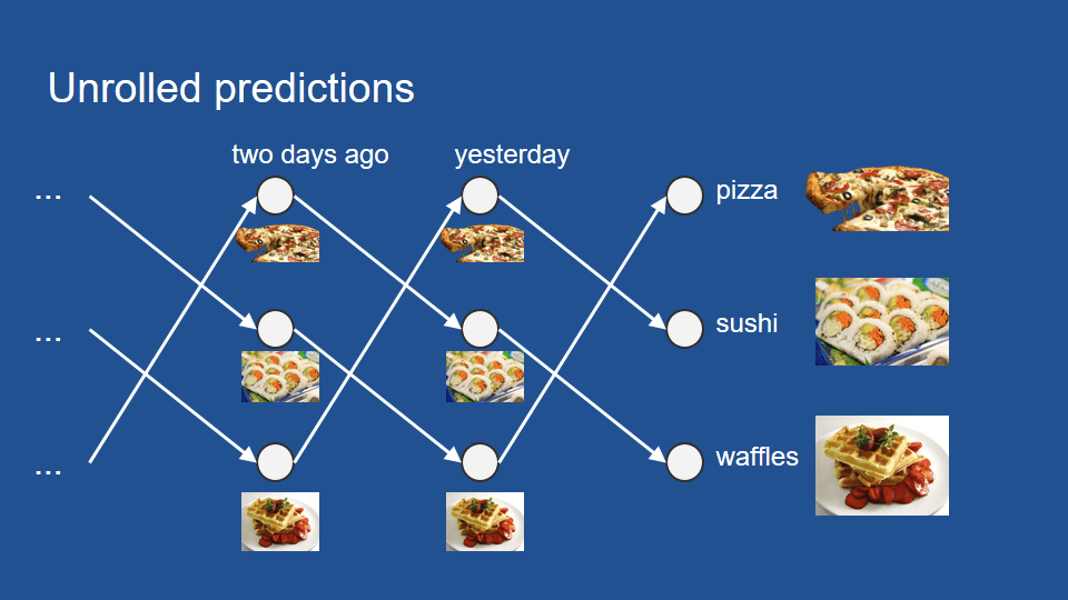
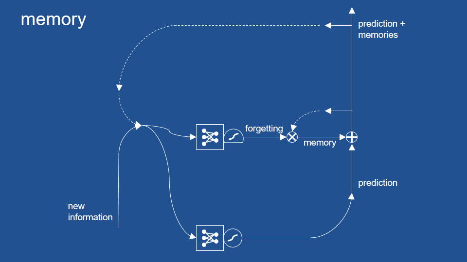
- the only Neural Network with memory and double data processing
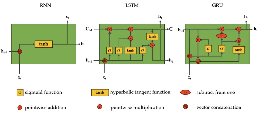
- Long Short-Term Memory (LSTM): uses short-term memory processes for creating long-term memory. It’s used mainly in Deep Learning, e.g. for making predictions in speech recognition.
- Gated recurrent units (GRUs) : a long short-term memory (LSTM) with a gating mechanism to input or forget certain features, but lacks a context vector or output gate, resulting in fewer parameters than LSTM.
- Feedforward Neural Network (FFNN)
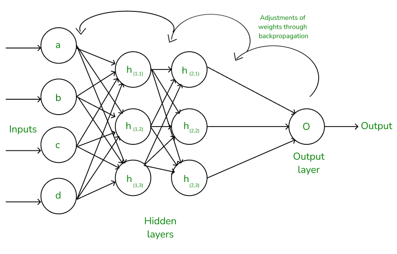
- Backpropagation
- Backward Propagation of Errors
- to reduce the difference between the model’s predicted output and the actual output by adjusting the weights and biases in the network
- Heavily used in feed-forward networks
- uses optimization algorithms like gradient descent or stochastic gradient descent. The algorithm computes the gradient using the chain rule from calculus allowing it to effectively navigate complex layers in the neural network to minimize the cost function.
- Activation Function
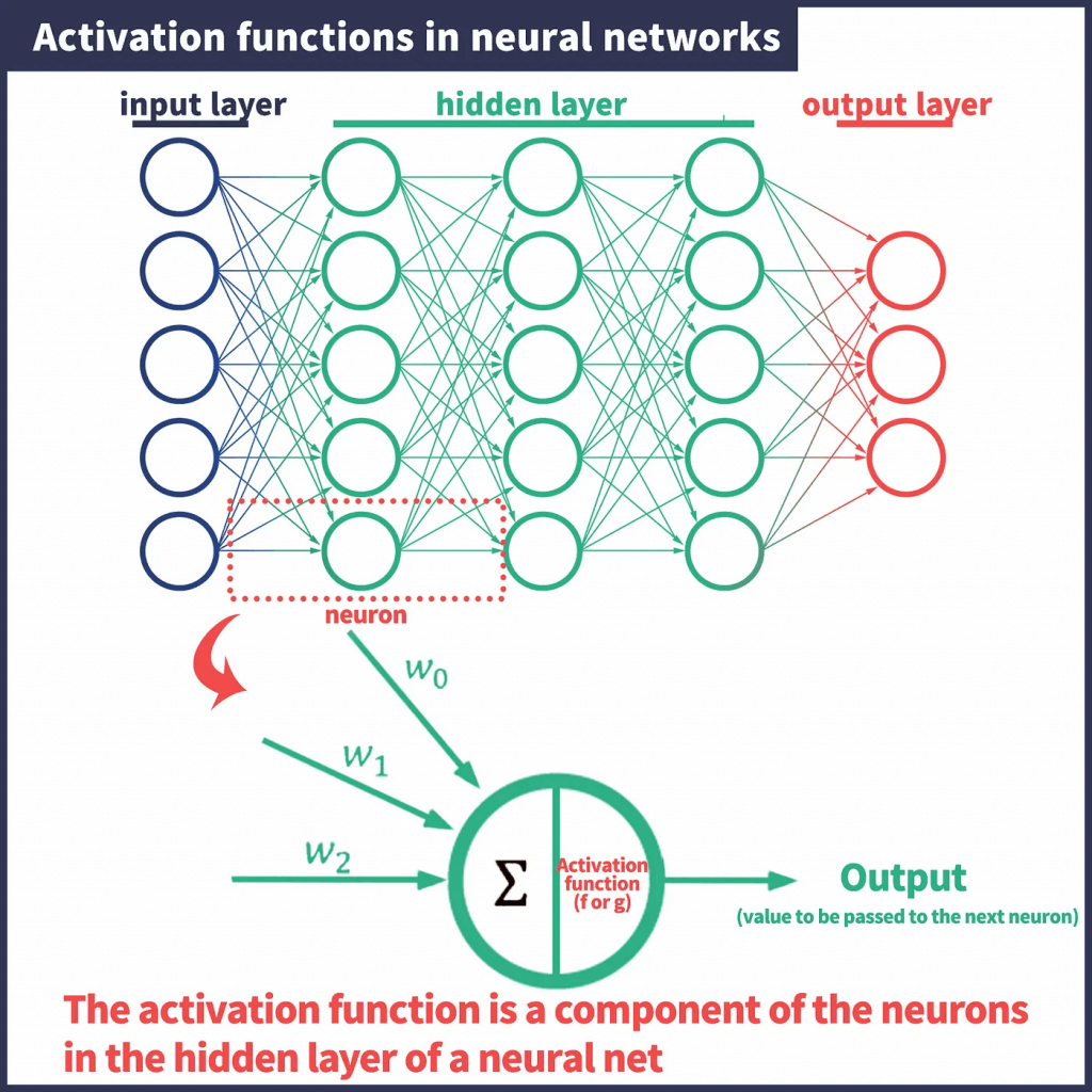
- The elements that make up the hidden layers of this neural network are neurons. Furthermore, one part that makes up that neuron is the activation function.
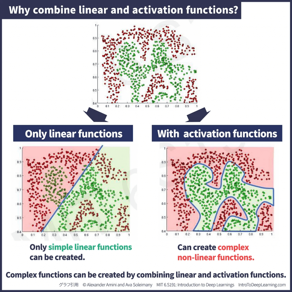
- each of the neurons that make up a neural network is made up of “a combination of a linear function and an activation function.
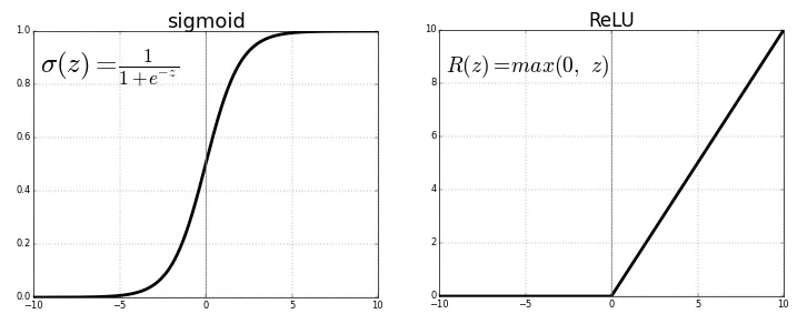
- The activation function works by outputting a value close to 0 if the input (the result of a linear function calculation) is small, and a value close to 1 if the input is large.
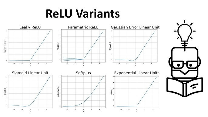
- Rectified Linear Unit (ReLU)
- Dying ReLU Problem: all the values less than zero will be zero after passing through the ReLU function. If the neural network is having a lot of negative values in the dataset then they all will be converted to zero after passing through the ReLU activation function and there will be zeros in the output which will make the neurons inactive.
- Variants
- Leaky ReLU (LReLU), for example, F(x) = max(0.01x, x)
- Parametric ReLU (PReLU), for example, F(x) = max(ax, x)
- Exponential Linear Unit (ELU)
- Scaled Exponential Linear Unit (SELU)
- Swish, useful in deep networks with 40+ layers
- MaxOut is a generalization of the ReLU and the leaky ReLU functions. It is a piecewise linear function that returns the maximum of the inputs, designed to be used in conjunction with dropout. Both ReLU and leaky ReLU are special cases of Maxout.
- has many Ws, and it is max(W1_T x + b1, W2_T x + b2, …)
- Softmax
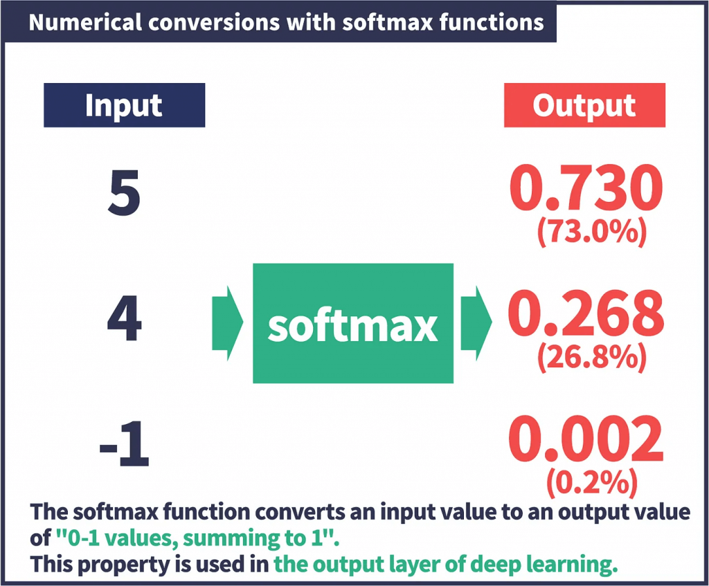
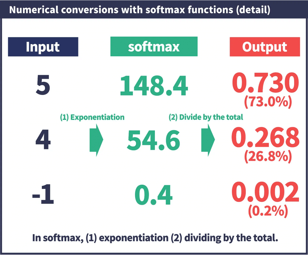
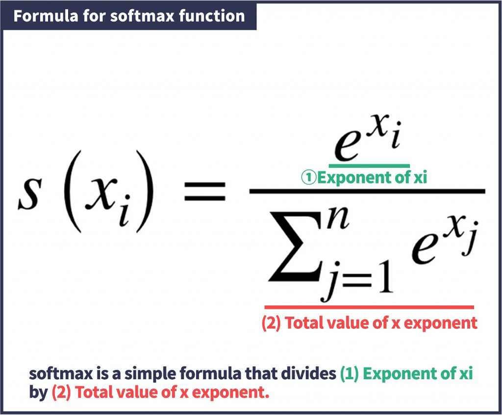
- a function that converts input values to 0–1 values that sum up to 1; ie, converts outputs to probabilities of each classification
- an “interpreter between AI and people”. Softmax functions are mostly used in the “final layer,” where the output values produced by AI are finally converted.
- Used on the final output layer of a multi-class classification problem
- How to choose Activation Functions?
- For multiple classification, use softmax on the output layer
- RNN’s do well with Tanh
- For everything else
- Start with ReLU
- If you need to do better, try Leaky ReLU
- Last resort: PReLU, Maxout
- Swish for really deep networks
CNN
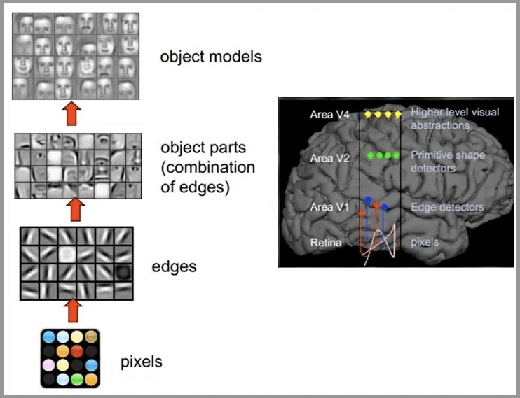
- preserves the characteristics of the image in a visually similar way. When the image is flipped, rotated or transformed, it can effectively recognize similar images.
- Typical parts
- Convolution layer
- extracting local features in the image
- Pooling layer
- significantly reduce the parameter magnitude (dimension reduction)
- Fully connected layer
- similar to the traditional neural network portion and is used to output the desired result
- Convolution layer
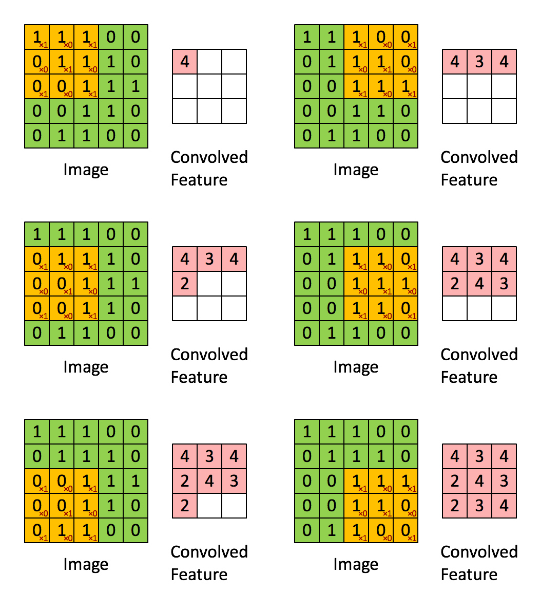
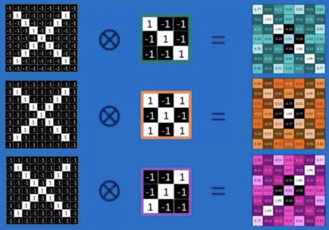
- Convolution
- using kernel (aka filter) to scan entire picture to get the convolved feature (aka feature map)
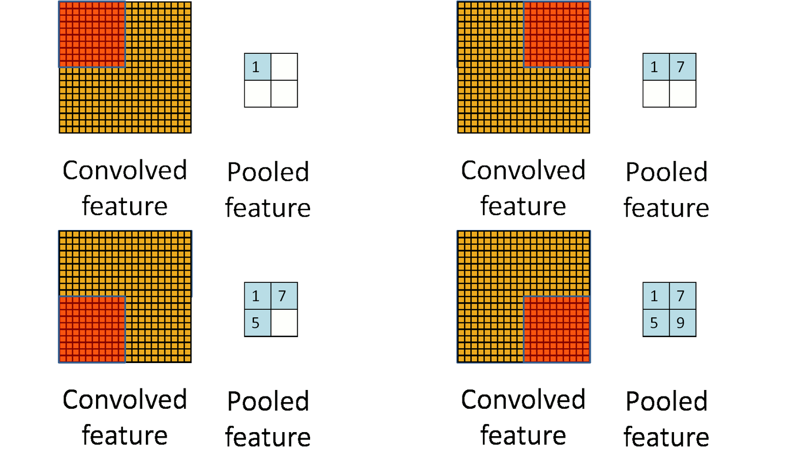
- Pooling
- as downsampling, to reduce data dimensionality to avoid overfitting
- Practical applications
- Image classification, retrieval
- Target location detection
- Target segmentation
- Face recognition
- Skeletal recognition
- Keras / Tensorflow
- Source data must be of appropriate dimensions
- ie width x length x color channels
- Conv2D layer type does the actual convolution on a 2D image
- Conv1D and Conv3D also available – doesn’t have to be image data
- MaxPooling2D layers can be used to reduce a 2D layer down by taking the maximum value in a given block
- Flatten layers will convert the 2D layer to a 1D layer for passing into a flat hidden layer of neurons
- Typical usage:
- Conv2D -> MaxPooling2D -> Dropout -> Flatten -> Dense -> Dropout – Softmax
- Source data must be of appropriate dimensions
- Specialized CNN architectures
- Defines specific arrangement of layers, padding, and hyperparameters
- LeNet-5
- Good for handwriting recognition
- AlexNet
- Image classification, deeper than LeNet
- GoogLeNet
- Even deeper, but with better performance
- Introduces inception modules (groups of convolution layers)
- ResNet (Residual Network)
- Even deeper – maintains performance via skip connections.


RNN
- Suitable for
- Time-series data
- When you want to predict future behavior based on past behavior
- Web logs, sensor logs, stock trades
- Where to drive your self-driving car based on past trajectories
- Data that consists of sequences of arbitrary length
- Machine translation
- Image captions
- Machine-generated music
- Time-series data
- Topologies
- Sequence to sequence
- predict stock prices based on series of historical data
- Sequence to vector
- words in a sentence to sentiment
- Vector to sequence
- create captions from an image
- Encoder -> Decoder
- Sequence -> vector -> sequence
- machine translation
- Sequence to sequence
- LSTM Cell
- Long Short-Term Memory Cell
- Maintains separate short-term and long-term states
- GRU Cell
- Gated Recurrent Unit
- Simplified LSTM Cell that performs about as well
| Parameter | RNN (Recurrent Neural Network) | LSTM (Long Short-Term Memory) | GRU (Gated Recurrent Unit) | Transformers |
|---|---|---|---|---|
| Architecture | Simple structure with loops. | Features memory cells along with input, forget, and output gates. | Merges input and forget gates into a single update gate; fewer parameters overall. | Utilizes an attention-based mechanism without recurrence. |
| Handling Long Sequences | Struggles to maintain long-term dependencies due to vanishing gradients. | Excels in capturing long-term dependencies due to memory cells. | Better than RNNs but slightly less effective than LSTMs for long-term dependencies. | Effectively manages long sequences using self-attention mechanisms. |
| Training Time | Quick but less accurate for complex relationships. | Slower because of more gates and memory operations. | Faster than LSTMs but slower than RNNs due to gating mechanisms. | Requires substantial computational resources but is highly efficient. |
| Memory Usage | Low memory requirements. | Higher memory consumption due to its complex architecture. | Lower memory usage compared to LSTMs, but more than RNNs. | High memory usage due to multi-head attention and feed-forward layers. |
| Parameter Count | Fewer parameters overall. | More parameters than RNNs because of gates and memory cells. | Fewer parameters than LSTMs due to its simplified gating structure. | A large number of parameters, especially in multi-head attention layers. |
| Ease of Training | Prone to vanishing gradients, making it harder to train on long sequences. | Easier to train for long sequences due to effective gradient management. | Simpler than LSTMs and easier to train than RNNs while maintaining performance. | Requires significant computational power and require GPUs. |
| Use Cases | Suitable for simple sequence modeling like stock prices. | Ideal for time-series forecasting, text generation, and tasks requiring long-term dependencies. | Similar applications as LSTM but preferred when computational efficiency is crucial. | Best suited for NLP tasks like translation, summarization, computer vision, and speech processing. |
| Parallelism | Limited parallelism due to sequential computation constraints. | Same limitations as RNNs; sequential processing restricts parallelism. | Same limitations as RNNs; sequential processing restricts parallelism. | High parallelism enabled by the attention mechanism and non-sequential design. |
| Performance on Long Sequences | Poor performance on long sequences. | Good performance on long sequences. | Moderate to good performance on long sequences. | Excellent performance on long sequences. |
Deep Learning on EC2 / EMR
- Appropriate instance types for deep learning:
- P3: 8 Tesla V100 GPU’s
- P2: 16 K80 GPU’s
- G3: 4 M60 GPU’s (all Nvidia chips)
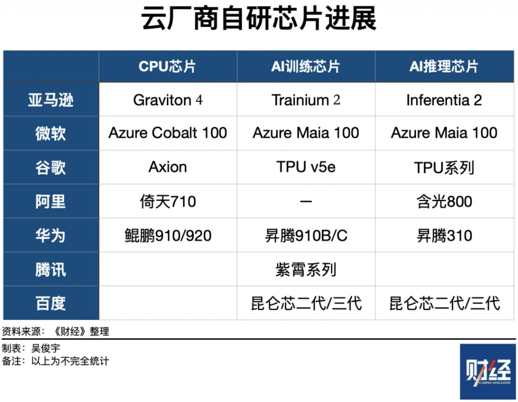
- G5g: AWS Graviton 2 processors / Nvidia T4G Tensor Core GPU’s
- Not (yet) available in EMR
- Also used for Android game streaming
- P4d – A100 “UltraClusters” for supercomputing
- Trn1 instances
- “Powered by Trainium”
- Optimized for training (50% savings)
- 800 Gbps of Elastic Fabric Adapter
- (EFA) networking for fast clusters
- Trn1n instances
- Even more bandwidth (1600 Gbps)
- Inf2 instances
- “Powered by AWS Inferentia2”
- Optimized for inference
Tuning Neural Networks
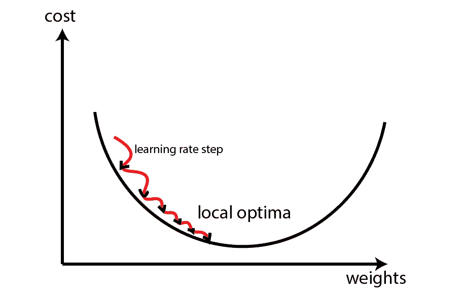
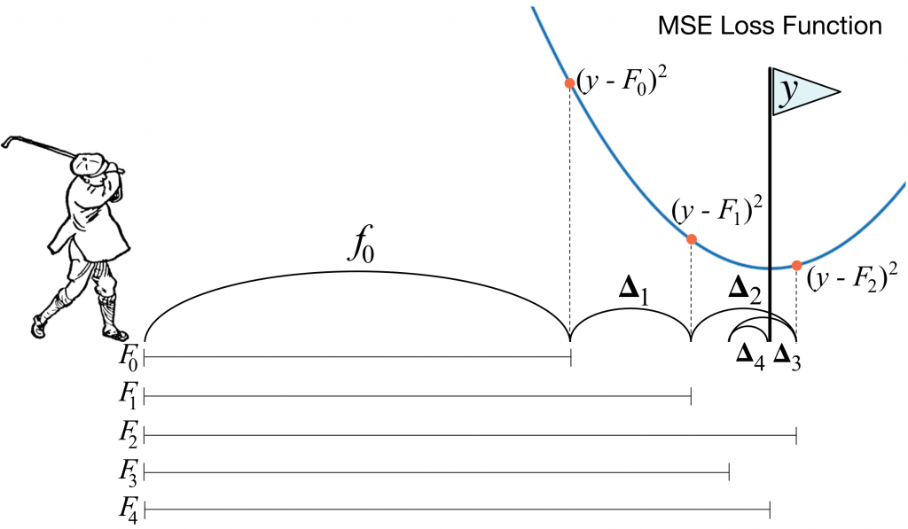
- Neural networks are trained by gradient descent (or similar means)
- We start at some random point, and sample different solutions (weights) seeking to minimize some cost function, over many epochs
- Learning Rate (the change of weights)
- How far apart of weights among epochs ; as an example of a “hyperparameter”
- Small learning rates increase training time
- Large learning rates can overshoot the correct solution
- Batch Size
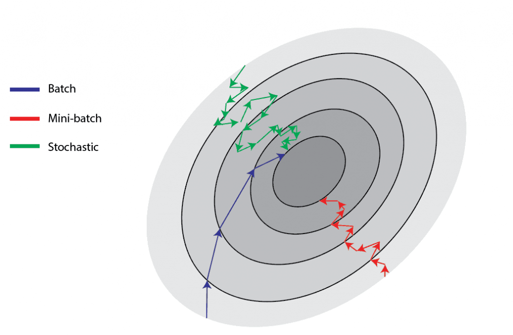
- How many training samples are used within each batch of each epoch
- Small batch sizes tend to not get stuck in local minima ???
- Large batch sizes can converge on the wrong solution at random
- Random shuffling at each epoch can make this look like very inconsistent results from run to run
- Regularization
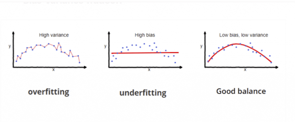
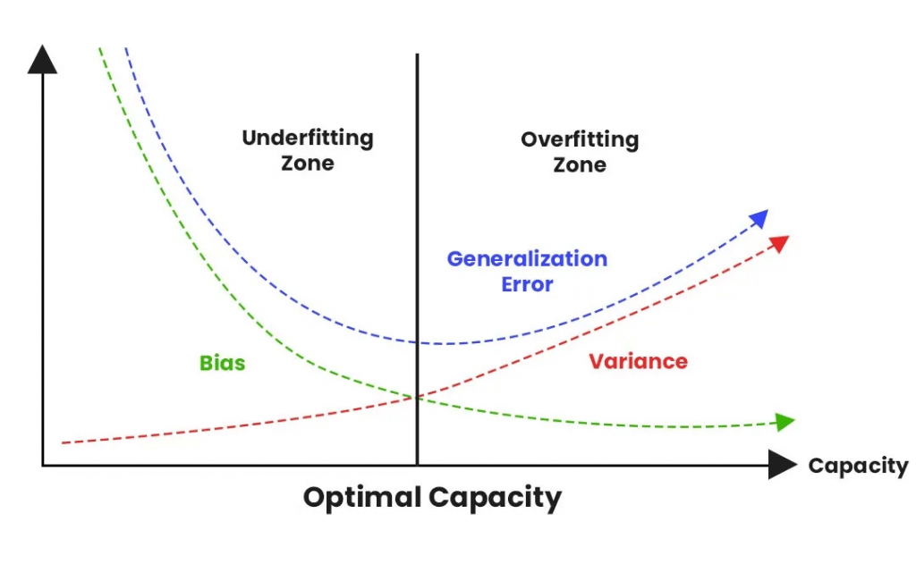
- Preventing overfitting
- Overfitting: models are good with training data, but not good at (unknown) new data
- Often seen as high accuracy on training data set, but lower accuracy on test or evaluation data set.
- When training and evaluating a model, we use training, evaluation, and testing data sets.
- Dropout
- Early Stopping
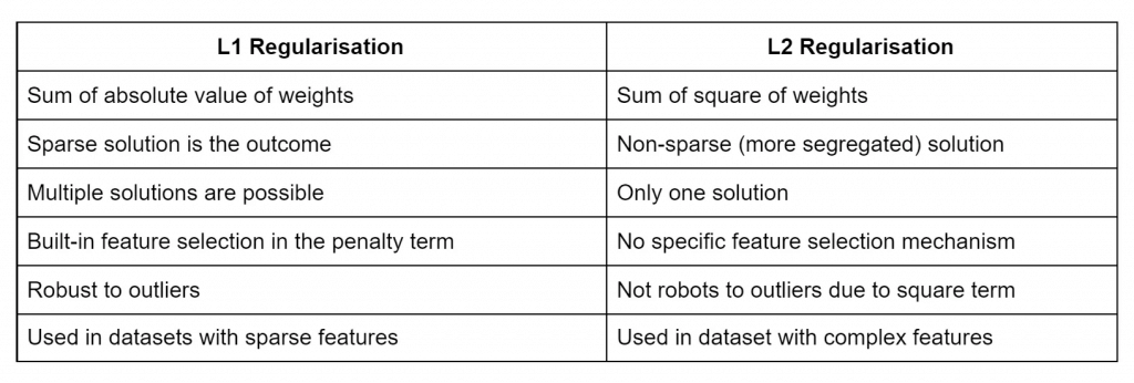
- L1 and L2 Regularization
- A regularization term is added as weights are learned
- L1 term is the sum of the weights “absolute”
- lasso regression, adds the absolute value of the sum (“absolute value of magnitude”) of coefficients as a penalty term to the loss function.
- Performs feature selection – entire features go to 0
- penalizing the weights to approximately equal to zero if that feature does not serve any purpose in the model.
- Computationally inefficient
- Sparse output
- robust in dealing with outliers
- Feature selection can reduce dimensionality
- Out of 100 features, maybe only 10 end up with non-zero coefficients!
- The resulting sparsity can make up for its computational inefficiency
- L2 term is the sum of the “square” of the weights
- ridge regression, adds the squared sum (“squared magnitude”) of coefficients as the penalty term to the loss function.
- All features remain considered, just weighted
- Computationally efficient
- Dense output
- not robust to outliers
- weights are of roughly equal size
- learn complex data patterns
- if all of your features are important, L2 is probably a better choice
- Preventing overfitting
- Grief with Gradients
- Vanishing Gradient Problem
- When the slope of the learning curve approaches zero, things can get stuck
- We end up working with very small numbers that slow down training, or even introduce numerical errors
- Becomes a problem with deeper networks and RNN’s as these “vanishing gradients” propagate to deeper layers
- Opposite problem: “exploding gradients”
- Corrected with
- Multi-level heirarchy
- Break up levels into their own sub-networks trained individually
- Long short-term memory (LSTM)
- Residual Networks
- i.e., ResNet
- Ensemble of shorter networks
- Better choice of activation function
- ReLU is a good choice
- Multi-level heirarchy
- Gradient Checking
- A debugging technique
- Numerically check the derivatives computed during training
- Useful for validating code of neural network training
- Vanishing Gradient Problem
Confusion Matrix
- aka Error Matrix, or matching matrix
- Each row of the matrix represents the instances in an actual class while each column represents the instances in a predicted class, or vice versa – both variants are found in the literature. The diagonal of the matrix therefore represents all instances that are correctly predicted.
- Total population = P +N
- True Positive Rate (TPR) = Recall = Sensitivity (SEN) = Hit Rate = Completeness = TP / P = TP / (TP + FN) = 1 – FNR
- how well the model identifies true positives
- Good choice of metric when you care a lot, about false negatives, i.e., fraud detection
- False Negative Rate (FNR) = Miss Rate = Type II Error = FN / P = 1 – TPR
- False Positive Rate (FPR) = Type I Error = FP / N = 1 – TNR
- True Negative Rate (TNR) = Specificity (SPC) = Selectivitiy = TN / N = 1 – FPR
- True Positive Rate (TPR) = Recall = Sensitivity (SEN) = Hit Rate = Completeness = TP / P = TP / (TP + FN) = 1 – FNR
- Prevalence = P / (P+N)
- Positive Predictive Value (PPV) = Precision = Correct Positives = TP / (TP + FP) = 1 – FDR
- the quality of positive predictions
- Good choice of metric when you care a lot, about false positives, i.e., medical screening, drug testing
- False Omission Rate (FOR) = FN / (TN + FN) = 1 – NPV
- Positive Predictive Value (PPV) = Precision = Correct Positives = TP / (TP + FP) = 1 – FDR
- Accuracy (ACC) = (TP + TN) / (P + N)
- False Discovery Rate (FDR) = FP / (TP + FP) = 1 – PPV
- Negative Predictive Value (NPV) = FN / (TN + FN) = 1 – FOR
- Balanced Accuracy (BA) = (TPR + TNR) / 2
- F-Score = ( (1+b2) * Precision x Recall ) / ( (b2) Precision + Recall )
- when b = 1, ie F1-Score = 2 (PPV x TPR / (PPV + TPR)) = 2TP / (2TP + FP + FN)
- Threat Score (TS) = Critical Success Index (CSI) = TP / (TP + FN + FP)
- F-Score = ( (1+b2) * Precision x Recall ) / ( (b2) Precision + Recall )
- Root mean squared error (RMSE) is another Accuracy measurement
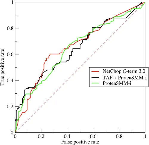
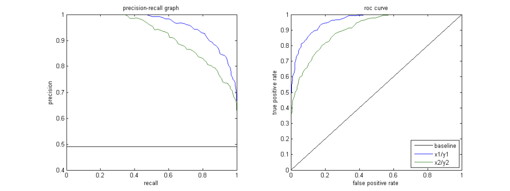
- Receiver Operating Characteristic Curve (ROC)
- Plot of true positive rate (recall) vs. false positive rate at various threshold settings
- Curve bent more on “upper-left” the better
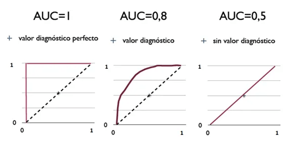
- Area Under the Curve (AUC)
- The area under the ROC curve
- probability that a classifier will rank a randomly chosen positive instance higher than a randomly chosen negative one
- ROC AUC of 0.5 is a useless classifier (Random), 1.0 is perfect
- P-R Curve
- Precision / Recall curve
- Good = higher area (PR-AUC) under curve, ie more “upper-right” the better
- When to use
- Imbalanced Datasets: When the positive class is rare, and the dataset is heavily imbalanced, the PR curve is more informative than the ROC curve.
- Examples include fraud detection and disease diagnosis.
- Costly False Positives: If false positives are more costly or significant than false negatives, such as in spam email detection, the PR curve is more suitable as it focuses on precision.
- Imbalanced Datasets: When the positive class is rare, and the dataset is heavily imbalanced, the PR curve is more informative than the ROC curve.
| Predicted condition | |||
| Total population = P + N | Positive (PP) | Negative (PN) | |
| Actual condition | Positive (P) | True positive (TP) | False negative (FN) |
| Negative (N) | False positive (FP) | True negative (TN) | |
Ensemble Learning
- In statistics and machine learning, ensemble methods use multiple learning algorithms to obtain better predictive performance than could be obtained from any of the constituent learning algorithms alone
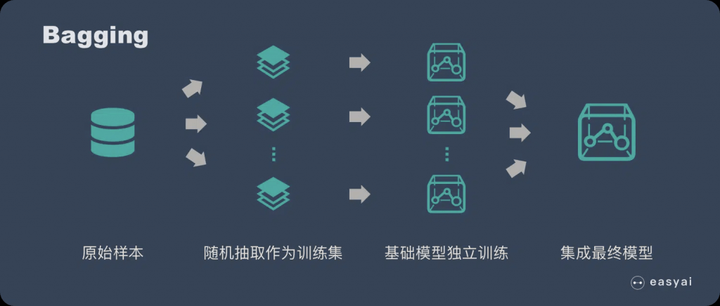
- Bagging (Bootstrap Aggregating)
- Generate N new training sets by random sampling with replacement
- Each resampled model can be trained in parallel
- The idea of Bagging is that all the basic models are treated consistently, and each basic model has only one vote in hand. Then use the democratic vote to get the final result.
- most of the time,The resulting variance is smaller after bagging.
- Example, Random Forest
- Boosting
- Observations are weighted
- Some will take part in new training sets more often
- Training is sequential; each classifier takes into account the previous one’s success.
- The most essential difference between Boosting and bagging is that he does not treat the basic model consistently. Instead, he tries to select the “elite” through constant testing and screening, and then gives the elite more voting rights. The poorly performing basic model gives Less voting rights, then combined with everyone’s vote to get the final result.
- most of the time,The result bias (bias) obtained by boosting is smaller.
- Example, AdaBoost, Gradient Boosting
- Bagging vs. Boosting
- XGBoost is the latest hotness
- Boosting generally yields better accuracy
- But bagging avoids overfitting
- Bagging is easier to parallelize

Hyperparameter Optimization (HPO)
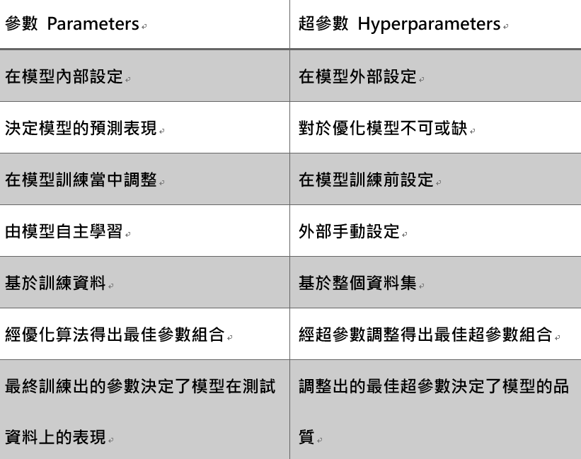
- A hyperparameter is a parameter whose value is used to control the learning process, which must be configured before the process starts
- Those hyperparameters are not possible to optimise during the process; for example, batch size, epochs, Learning Rates, K Neighbors, RNN step duration, …
- the problem of choosing a set of optimal hyperparameters for a learning algorithm.
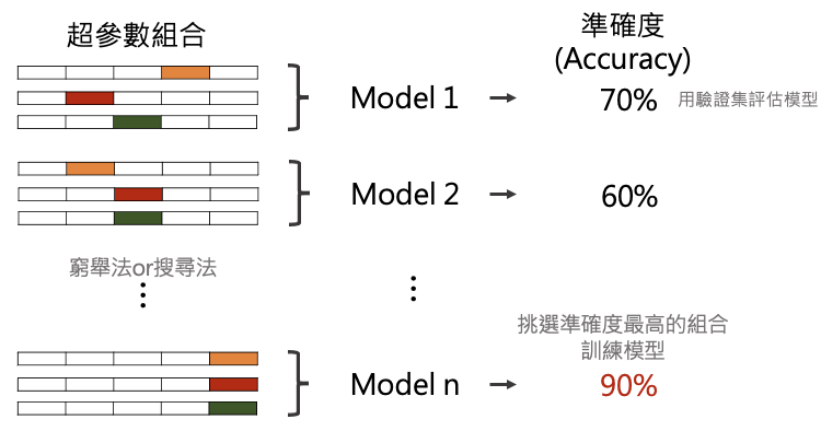
- Grid Search
- With grid search, you specify a list of hyperparameters and a performance metric, and the algorithm works through all possible combinations to determine the best fit. Grid search works well, but it’s relatively tedious and computationally intensive, especially with large numbers of hyperparameters.
- Random Search
- Although based on similar principles as grid search, random search selects groups of hyperparameters randomly on each iteration. It works well when a relatively small number of the hyperparameters primarily determine the model outcome.
- Bayesian optimization
- Bayesian optimization is a technique based on Bayes’ theorem, which describes the probability of an event occurring related to current knowledge. When this is applied to hyperparameter optimization, the algorithm builds a probabilistic model from a set of hyperparameters that optimizes a specific metric. It uses regression analysis to iteratively choose the best set of hyperparameters.
